Handling Duplicate Data

Handling Duplicate Data is well-known to be a Vexing Problem for many Excel users. 

There are tools within Excel that simply delete all duplicate data, but there are times when it is more advisable to Identify these Duplicate Values prior to eliminating them.

For instance, let's say you are working with Combined and Blended human resources data that lists employees with their home addresses. If the information in the blended data includes Duplicates of employees who have had updates, and shows different addresses for these duplicates, it would be good to have an Expedient Way of doing identifying them before taking action.

Conditional Formatting can offer an excellent solution:

1.   Select the range (e.g. A1:A98).

2.   Choose Format / Conditional Formatting to display the CF dialog box

3.   Select Formula Is from the first drop-down list box, and enter =COUNTIF($A$1:$A$98,A1)>1 in the second box

4.   Click the Format button to bring up the Format Cells dialog box.

5.   Select the Patterns tab, and choose a background color

6.   Click OK twice to return to your worksheet

Bamm! If the range contains any duplicate entries, they will be highlighted with the background color you chose previously!

Removing Duplicates in databases is one of the most infamous topics for many Excel professionals. Being able to do this, enables a user to Combine Databases with repetitive data into a properly structured format.

With the last three versions of Excel (2007, 2010, and 2013), this is Remarkably Easy. Here is all you have to do to complete this simple task:

1.  Select the entire database (be careful not to select any self-generating key fields)

2.  Go to the Data tab in the Data Tools group and click Remove Duplicates

3.  Select the column(s) on which you want to base your removal and click OK

4.  A message will pop up telling you how many (if any) values were found and removed

At first glance Removing Duplicates to maintain the Integrity of your data may seem like a challenging task. As is the case with nearly everything in Excel, however, once you know how to do it, it seems so Comparatively Simple, you may wonder why you ever considered it a problem…

Why to Use AutoCorrect...

“I Haven’t Got Time to Save Time”. You may not have ever heard or said these words, but the fact is that many people conduct their professional lives as if this phrase were the mantra to their philosophy.

Being an Excel Enthusiast, you naturally believe there are easier ways to do things, and that brings to today’s subject, AutoCorrect!

If you routinely need to type out a Company Name or any other so-called “Boilerplate” text in Either Excel or Word, you can Save Time by setting up your AutoCorrect option to Automatically change the text you are writing.

Of course, AutoCorrect is initially set up with a list of typical misspellings and symbols, but this is for the everyday masses, not Excel Gurus such as yourself! Let’s say you work for National Public Radio, and the legal department wants the entire name of your service Spelled Out each time it is entered into a worksheet.

While this may seem like a chore, AutoCorrect can make this is as easy as typing NPR.

Here is How You can Set this Up:

1. Go to FILE and select Options from the bottom of the column

2. Choose Proofing and click on the AutoCorrect Options button

4. In the Replace box, type NPR

5. In the With box, type National Public Radio

6. Click Add and then OK That’s all there is to it! But wait! There is also a World of Opportunities to have a little Fun as well!

Let’s say you have a friend named Gary at work (any name will do). While he is away from his computer, go into AutoCorrect and enter Gary in the Replace box and Geek Boy in the With box.

Do this in Word also, and he will be stunned every time he types his name! This is great adolescent fun, (but it helps if you know Gary has a sense-of-humor…). Just be sure you have him do this in your presence, so he doesn’t unnecessarily embarrass himself (and you).

Using AutoCorrect can better your life. Unless, of course, You don’t have Time to Save Time…

Embedding Excel in Other Programs

We all agree that Excel is the Quintessential Tool for crunching numbers and developing corporate information. There are times, however, when you may want to Upgrade the way you present your findings to the stakeholders of the data.

If, for instance, you are making a presentation with PowerPoint, it is typically much more effective if you insert your Excel information, (a chart, for instance), rather than having to switch programs midstream.

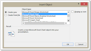
To do this, simply open a PowerPoint presentation (or Word document if that suits your purposes) to add the Excel worksheet, then Insert Object. Choose Microsoft Excel Chart from the Object Type and click OK.

 

You will instantly have a generic Excel chart inserted into your presentation or document. From there, it is equally easy:

• Just right-click the chart and choose Edit Data from the dropdown list. You can import it from a worksheet you have already created or, if you choose, create your own data on the spot.

• Changing the Chart Type can also be accomplished from the same dropdown, as can formatting (Format Chart Area…)

• If you want to save the chart image as a static image, you can choose Save as Picture and save to a file, locking in all that you have done for possible future use.

By using these tools, you can enhance that overt Professionalism in your presentations and documents. Very cool!

Excel Wizardry

As with so many things in life, what seems like “Wizardry” in Excel is really a matter of knowing some Simple, albeit powerful, Tricks.

#1 - Multiple Lines of Text within a Cell
Have you ever wanted to add multiple lines of text to an individual cell? How can this be done, you ask? The answer is so easy, you’ll laugh.

When you want to insert a line break within a cell to break up your text for readability, just hold down Alt and hit Enter. You are also turning on Wrap Text when you do this. Cool!

#2 - Delete Blank Rows
If you have blank rows of cells within your database or table, it can potentially cause issues when deriving information (and who needs that…). Select a column, press F5, click on Special, select the Blanks option, and click OK.

Now that you have the blanks targeted, click over to Excel’s Home tab and go to the Cells group. Select Delete Sheet Rows and Bamm, no more blanks!

#3 – When Numbers are Not Numbers
Excel will occasionally store numbers like a “0” as Text instead of a numeral, (often when importing from another program). This can be problematic, especially if you have a sizeable database. The solution, once again, is so easy you’ll laugh!

  First, simply type a “1” into an empty cell outside of you data. Select and copy it to your clipboard, and then select the range of numbers you wish to fix. Right-click and choose Paste Special, select Multiply, and click OK. Problem Solved!

Simple tricks that look like Wizardry. Everything is simple when you know how!

Errors, Errors, Everywhere!

We’ve all Been There, Done That. You are creating an Excel masterpiece formula when you are troubled, nagged, and thoroughly bugged by some Error Messages.

The following is a handy Alphabetical Listing of Error Messages and what they mean:


• #DIV/0! - You divided by 0 or by an empty cell (Everyone knows you can’t do that…)
• #N/A - A return value of the function is not available (You probably messed up the formula)
• #NAME? - Okay, you might have used an undefined range or cell name (easily corrected…).
• #NULL! - You specified an intersection of two areas that do not intersect (Curious error…).
• #NUM! - There is a problem with a number in a formula (Is it really a number?).
• #REF! - An invalid cell reference is mentioned in a function (A cell reference is not valid).
• #VALUE! - The wrong type of argument or operand is used in the formula (Yeah, yeah, yeah)

Now let’s look at a few Handlers you can use to Attack Errors:

1.   ISERR - Any error value except #N/A
2.   ISERROR - Any error value, including #N/A, #VALUE!, #REF!, NAME?, etc
3.   IFERROR – Introduced in Excel 2007, this combines the IF and ISERROR functions

Let’s use the IFERROR in an example. Suppose you have two columns of data which you are simply dividing in a third column. If you Divide by 0 or Divide by a Blank Cell, you will obviously get an Error Message.

 If, however, you want the message to be Perfectly Clear, (as our former President Nixon was fond of saying…), you use IFERROR to define a Custom Response such as “Error in Calculation” or “Problem with 2nd Value”, or something more clever that you invent for your circumstances. In the example shown, the formula would be:

 =IFERROR (Column_1 / Column_2, “Error in Calculation”)

By not simply accepting Errors and Error Messages, you can better Take Control of your Excel workbooks. Always a good thing…

Macro Robots

Although the topic of Excel Macros is a bit overly ambitious for a blog of this type, it is a subject about which many individuals are interested. Macros are not part of most Excel users skillset, but they can help make your day-to-day tasks much easier and the basics should not be intimidating.

Many of us have workbooks which we need to continually update with new data and repeat certain tasks over and over. A Recorded Macro can be your ticket to lessening your repetitious work and simplifying your routine chores.

A Macro can record your mouse clicks and keystrokes while you work, and then allows you to play them back in future renditions of your workbook. When you run the macro, it will play the commands in the same order that you recorded them. It’s like having a Macro Robot at your command!

For example, let’s say you track the performance of the representatives in a call center. Every week a report must be created for management, and it involves routine updates. Here's how to record a macro to apply these updates:

1.   In the report workbook, click the start of the cells you are going to update.
2.   Point to the Developer tab, and then click Record Macro.
3.  In the Record Macro dialog box, enter a Name that applies to your operation. For ease of operation later on, assign a custom Shortcut Key.
4.   Now perform the calculations, formatting, moving, etc that applies to the repetitive and monotonous update.
5.   Finish recording the macro by clicking the Stop Recording button.

To Run your Macro, simply go to the update start cell and enter your Custom Shortcut Key.

Bamm! Instant update! Your newly created Macro Robot has just done all of the work that may have taken you several minutes or an hour to complete. Give it a try – Totally worth the effort!

Give Me the Green Light!

Let’s face it, Excel worksheets can at times be a Bit Drab. A worksheet can serve as a Decision Tool and showing a Yes, No, or Maybe next to your agenda items can get the job done, but it’s really Ho-Hum, isn’t it? Since the introduction of Excel 2007 you have some very interesting options, however. You can use sets of Graphical Icons with your decision lists, and give your reports some Much Needed Life!

For an example, let’s suppose we have a proposed agenda for an upcoming annual corporate meeting. Possible topics have been submitted from numerous sectors, and you want to use a Semaphore for an icon when make a preliminary worksheet showing a:

• Green Light for a definite inclusion in the program
• Yellow Light for a possible inclusion
• Red Light to exclude the topic from the agenda

Here is How to Accomplish This:

1.  Select the range of cells in which you want a Semaphore to appear
2.  Click Conditional Formatting on the Home tab, choose Icon Sets and pick the set that includes the Semaphore
3.  Go back to Conditional Formatting and choose Manage Rules
4.  Click Edit Rule and put a check in the Show Icon Only box and Apply
5.  By default, a “1” will be a Red Light; “2” will be a Yellow Light, and “3” will be a Green Light

Your Decision Lists will instantly take on a New, Engaging Look and will be sure to garner the closer interest of any of the users. And, of course, the cool thing is that it is Easy (Isn’t anything when you know how…).