Use Conditional Formatting to Highlight Above-Average Values

Highlighting exeptional values can be a useful (and simply-done) analysis tool. Here is an easy way to highlight the Above-Average values in a range:

1. At the bottom of your range, enter the formula for Average: =Average(range)
2. Select the values in the range (not including the Average formula)


3. On the Home tab in Excel 2007, choose Conditional Formatting from the Styles menu


4. Select Highlight Cells Rules / Greater Than


5. Choose the dialogue box and click on the cell in which you have the Average Formula


6. Choose the Formatting you wish to apply


7. Click Enter and Presto! Values that are Above-Average are highlighted!
   

Use this simple method to highlight Above-Average values (You will be Above-Average Yourself!)

Right-click Tab Scrolling Buttons

Large Excel workbooks will commonly contain a great many worksheets that can be cumbersome to scroll through to find a particular item.

A quick and easy shortcut to the worksheet of your choice is to right-click the tab scrolling buttons in the lower-left corner of your workbook. A menu will appear showing the tab names. You can then choose your location and navigate to it directly.

Bamm! You can go right to your worksheet and skip by the rest!

Quick Chart!

This has always been one of my favorite easy crowd-pleasers.

To make a Quick Chart, simply select your table of date, and press F11. Bamm! A full-featured chart will be inserted in your workbook. Don't like the default chart? Just right-click the resulting chart and choose Change Series Chart Type.

Give it a try, and listen to them go "Oooh and Ahhh..."

Beware: There May be Links in this Workbook!

If you are working within an Excel document that you may not be familiar with, be cautious before deleting or clearing a cell containing a formula. You can use the keyboard shortcut for revealing another cell that it may be feeding by pressing Ctrl + Shift + ] (Closing Bracket).

If it doesn’t reveal any linked cells, you can safely delete the formula (Cool!).

Favorite Keyboard Shortcuts

Keyboard Shortcuts can add speed, comfort, and enjoyment to your Excel experience. Although there are dozens, (you probably use some already), the following three are some of my favorites:

1. Control/h: I often need to find and replace the information in a range of cells. This one makes it quick and easy.

2. F5: This allows you to pick a named range from a list and transport you there immediately.

3. F11: Impress your colleagues by selecting a table of information and creating and instance chart. Fun stuff!

Keyboard shortcuts are not only time-savers, they’re Cool as well!

Obtaining a List of Unique Names

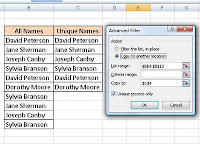
Obtaining a list of Unique Names is often a beneficial function in Excel. The good news is that it is Easy!

First, select the original range of names (See column 'B' All Names).

Second, go to Advance Filter, choose Copy to and select a cell for the starting point.

Lastly, check the checkbox for Unique Records Only and click OK.

Bamm! A list of Unique Names! Give it a try...

Naming Ranges: Why & How

Why
Naming ranges in Excel can save you a lot of time and make your formulas more intuitive.
Using a named range in a formula does away with the need to make the range an absolute reference because it will always point to the correct range, regardless of where you copy the formula.

How

1. First highlight the range of cells you wish to name
2. Now click inside the “Name” box on your toolbar at the upper-left of your screen
3. Type your chosen name for the range
4. Hit the Enter key and Presto! Your range is named. Give it a try!
   

Using Comments

Adding comments to specific cells in an Excel worksheet can help the user determine the meaning of the data. This can be particularly useful if the user is not the creator of the worksheet.

Using Comments:
1. Select the cell in which you want the comment
2. Right-click and choose Insert Comment
3. Type your comment
4. When finished, click outside the comment box
5. The red triangle in the upper-right corner denotes a cell with a comment
6. To view a comment, simply hover your mouse over the cell

Inserting comments is easy and very useful. Give it a try!

Creating a DropDown Box with Validation

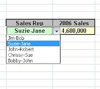
Using a DropDown Box in an Excel report can add interactivity, efficiency, and a professional style to your worksheet.

A easy and effective way to do this is by using Validation. Simply select the cell in which you want the dropdown, (such as the green-shaded cell in the graphic), choose Validation / Allow List and then select a range for your Source of dropdown entries.

Presto! Instant DropDown Box!

By combining a dropdown and elements such as a VLookup function, you can create a powerful and interesting report in Excel.

Stock Quote Reports in Excel

So, you want reports on your Stock Portfolio delivered into Excel, do you?

1) Select cell A1
2) Go to Data / Get External Data / Run Saved Queries,(this may differ slightly depending on Excel version), and choose Microsoft Investor Stock Quotes
3) Enter some stock symbols (eg. UTR, MSFT, GM, etc.) and click "OK"

Presto! In a few seconds, you will have all of the current data on your stocks!

Welcome to the Excel Enthusiasts Blog!

Hello Excel Fans!

Today marks the debut of the Excel Enthusiasts blog! In the weeks and months ahead, this blog will explore all (or a whole lot of...) things Excel. Topics will range from common, routine procedures in this application to truly esoteric, wild and wonderful looks at what this powerful tool can do.

I hope you will check in now and then. You can also join the Excel Enthusiasts Group on LinkedIn and stay connected with other Excel afficiandos!

All the best,

Bob (The Excel Guy)