Navigating on Excel

Readers of this blog have said they would like to occasionally return to some of the basics, so today we are going to review the topic of navigating in Excel.

Sailing the seas of your Excel worksheets can be chore unless you know a few simple tricks. For instance, if you wish to go to your last entry at the bottom of a list that contains 30 records, scrolling to where you wish to go is simple and effective. When you have a list containing 3,000 records, however, it is a bit tedious.

As is true with so many Cool Moves in Excel, keyboard shortcuts rule when it comes to saving time moving from one location to another on your spreadsheet.

Here are few Cool Moves you can make without ever touching a mouse:

1. Control / Down Arrow: Goes to last cell in column with data

2. Control / Right Arrow: Goes to last cell in row with data

3. Control / End: Goes to last row, column and cell

4. Control / Home: Returns to cell A1

When using your mouse, another way to navigate to the end of your data (whether in a column or row) is to carefully place your pointer on the adjacent border of cell in your range and double-click. For instance, if you wish to navigate to the last cell in a column of data that starts with cell C1, you can select C1 and double-click on the bottom border of the cell.

Want one additional way to navigate when you know the exact address of some remote cell? Simply enter the address (e.g. ET3000) in the Name Box and Bamm; you have beamed directly to that location.

Try a few different ways of navigating on the Excel seas; you can sail to where you want to be in the blink of an eye!

Dynamic Chart Title (Oh, Wow!)

If you are looking for an “Oh, Wow!” feature for your next report containing a chart, the use of a Dynamic Chart Title is for you! By linking the chart title to a value displayed in a specific cell on your worksheet, you can create a very accessible chart that will amaze and delight your users.

As we have discussed before, it is super easy to create a dropdown list using Validation/List. If you have created a table that changes in accordance with the value shown in the dropdown, (e.g. a salesperson’s name), you can in turn create a chart that shows the updated data (e.g. a salesperson’s performance), along with the sales professional’s name in the title.

Here is how you do it:

1. Select the Chart Title
2. Go to the formula bar and type “ = ” and
3. Select the cell to which you want to link (be sure to use an absolute reference)
4. (Note: The final cell reference formula should look something like: “ =Sheet1!$B$2 ”

Oh, Wow! What a great way to add functionality, ease-of-use, and Pizzazz to your reports!

Happy Holidays, All!

When in Rome...

Once in a while, it is good to have a bit of geeky fun. Although of no real practical use, it can be interesting, (once again, in a geeky sort of way), to play around with Roman numerals. For an Excel user, it is particularly interesting to find that the application has a built-in Roman numeral function.

Practicality, of course, can be overrated, and it is readily apparent that Hollywood, Football, and the Olympics have all used Roman numerals on a regular basis. If you also wish to do this sometime in Excel, (I probably wouldn’t recommend it for your next quarterly report to your boss, unless the individual has a really good sense of humor), you can use the Roman function.

For a classic numeral, (other formats are available, but who needs them…), simply enter a value in cell A1 and type, “=Roman(A1)” in cell B1. Hit Enter and Presto, a Roman numeral of the A1 number! Now you will be all set if the NFL needs someone to come up with the name for the next Super Bowl!

Fun with the Spinner Buttons!

Since they control the data that can be entered and are easy-to-use, so-called “Spinner” buttons can be a clever addition to a spreadsheet. To add a spinner in Excel 2003 and in earlier versions of Excel, click the Spinner button on the Forms toolbar, and then draw your spinner on your worksheet. (You can size the Spinner to your liking.) To add a Spinner in Excel 2007, click the Developer tab, click Insert, and then click Spin Button in the Form Controls section.

Now you are all set to have some fun! Right-click on the spinner, and then click Format Control. On the Control tab complete the values as follows (this is a test, ma’am or sir, only a test…):

1. Current value: 1
2. Minimum value: 1
3. Maximum value: 10
4. Incremental value 1
5. Cell link: $C$7 (Note: Any of these values can be of your own choosing.)

Now when you click the Spinner control, cell C7 is be updated according to the parameters you set. If you have created a worksheet where other cell values or results are dependent on the value in C7, your worksheet will update according to the quantity you select with the Spinner.

How cool is that! Make your Excel worksheets look like someone spent hours of programming time on them in just 5 minutes. Give it a try (people will think you are a Star!).

Conditional Formatting Revisited

Good communication is the life blood and Bane of business. This fact could not be truer than in reports and presentations that involve numbers (Financial and Performance reports are notorious examples). Nothing causes the glazing of eyes like a large table of numbers with row after row of monotonous monotone data.

So how do we get our numerical information across to our stakeholders in an efficient and engaging manner? Well, although Charts are obviously very effective, they are not the only method. Conditional Formatting is a very powerful technique that should not be overlooked.

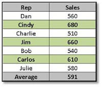
Taking a simple table of sales data as an example, let’s say that you would like to have your audience be able to easily identify those reps with sales greater than the average. First, create a simple formula in the last row that calculates the average of all sales, (e.g. “=Average(B2:8)”). Then set your Conditional Formatting for the first row to highlight (I like to choose my own formatting set to give it a bit of a custom look) if the value in the numerical column is greater than the cell displaying the average (=B2>$B$9).

Then it is a simple matter of selecting the cells with conditional formatting, clicking the Format Painter, and “painting” the rest of your table. Bamm! Instant impact and improved communication! This is Easy (and “Easy” is Good). Give it a try and brace yourself for Accolades…

Excel 2010 - More News!

Now that we are nearing 2010, you may be interested in what is going to be New and Cool in the latest release of Microsoft Excel 2010. Here is a brief overview of some of the new and/or improved features:

• Continued innovation in the charting engine, with features like “sparklines”, a better user-interface, cross-sheet conditional formatting, and improved interactivity.
• Improved Excel Web App experience, with many core features available in your favorite browser. Multiple users can now edit the same spreadsheet simultaneously.
• Speedier calculations with improvements in file load and charting that make Excel feel faster overall.
• New functions have been added, along with a new version of Solver.

I don’t know about you, but I can’t wait to get my geeky hands on a copy of the new Excel. Please let me know if you are one of the privileged few to get an advance copy. Cheers!

Add More Lines of Text in a Cell

Although the focus of Excel is numbers, there are times when you want to enter text into cells as well. Sometimes you may even want to add another paragraph (or perhaps just a line break) in a single cell. If you are working in Word, that’s easy – just hit the Enter key.

In Excel, however, hitting Enter will just take you to the next row below. “Bummer!” you say, but take heart, the solution is so easy it will make you laugh.

All you need to do is press Alt+Enter to start a new line in the cell in which you are typing or editing. That’s all there is to it! (See if you colleagues know that one…).

Viewing Excel on Two Monitors

Unlike MS Word, the great minds at Microsoft have chosen to not make the default ability to view different Excel workbooks simultaneously on two monitors. Since many of us use multiple monitors and would occasionally like to compare worksheets, this can be annoying.

Although you can mess around with the folder options in the Windows Tools, there is a very easy way to make Excel display to your liking. All you have to do is hold down on the CTRL key when you launch Excel for a second time and it will open a second instance that you can drag into a second window.

Yup! That’s all there is to it! If you use two or more monitors, give it a try sometime! It is easy and effective.

Using Goal Seek

"What If” scenarios are a valuable instrument for nearly any business. Excel provides a great tool to accomplish this by automatically making changes in a variable using Goal Seek (it can save you a ton of work, and make you look good in the process).

Using a very simple example, let’s say that you are a call center sales manager, and you know the approximate number of calls you are going to receive for the next month, as well as the sales goal that has been set by the executive branch. You wish to know the call-to-sale-conversion-rate so you can advise your staff. A rudimentary calculator can be created in the cells of your Excel worksheet as follows:

Number of Calls x Conversion Rate = Number of Sales (e.g. C4*C5 = C6)

After filling in the values for C4 and C6, you can use Goal Seek to calculate the required value for C5.

Obviously, this tool can be used to greater advantage with more complex scenarios, but you get the picture. Goal Seek can be a handy tool for the boardroom or any planning venue. Give it a try sometime!

Fresh Repetitive Data

Bob is back! Greetings to all of my fellow Excel Enthusiasts; It is so good to be back on the blog after an unavoidable absence.

Here is a great little technique that I recently ran across. Although it is very intuitive to copy and paste repetitive data to a set of noncontiguous cells (copy data, select the cells and paste), entering newly typed data doesn’t work quite that way.

To enter new data into a series of noncontiguous cells, simply hold down the Ctrl key and select all of the cells into which you want to enter your new data. Then type the text you want to enter and (drum roll, please…) press Ctrl+Enter.

Bamm! Excel will enter the typed text into all of the cells in your selection. (How cool!)

Calculate Car Payments

Okay, let’s say it is time to trash the Nerdmobile and buy a new car. Well, no self-respecting geek is going into a car dealer without his or her trusty laptop or netbook loaded with the most recent version of Excel.

Why is that, you ask? To calculate the monthly car payments, of course! Here is how:

The Excel PMT() function can calculate the monthly repayment using the following format:

PMT(AnnualInterestRate/12, NumberOfPayments, AmountOfLoan)

For example, if your annual interest rate is 6%, on a 5-year (60 months) loan of $30,000, your formula would look like this:

=-PMT(0.05%,60,30000)

Note that a negative sign (-) was placed in front of the function in order to return a positive value (negative payment values look messy…)

With your formula in place, hit Enter and, Presto, you have your monthly payment. If you don’t like the results, play around with the interest rate, the length of the loan, or maybe check out some cheaper cars. How cool!

Using and Creating Templates

Excel templates are files containing common data and formatting options used as models for other spreadsheets. A template is a great shortcut for standardizing the look and functionality of your data. Templates can also provide you with a standard framework in which to input and share your data. Reusable formulas and fields enable you to speed up your input and get the information that you want in the form you want.

Using a Template

1. Go to the File menu and choose New
2. Click on Templates and select the general category
3. Double-click on the desired template
4. A new worksheet opens and displays the template
5. Be sure to name the worksheet when you save it

Creating a Template:

1. Open a worksheet you want to use as the basis for the template
2. Choose Save As and enter a name for the template
3. From the Save as Type list, select Template
4. Save the file inside the Templates folder

That’s it! Try it out – Templates can save you a lot of work, and help you maintain a consistent, professional look.

Sorting Order – Have it Your Way

Although the innate sorting options in Excel are usually sufficient, there are times when you need a Special Sorting Order to fit your data. Never fear, you can easily create your own customized sorting orders.

For instance, if you have a field containing your corporate locations (let’s say Chicago is the home office, and the other locations are ranked according to production). You may want Excel to sort the locations as follows: Chicago, Minneapolis, Albuquerque, and Los Angeles. The problem is, of course, that Excel would typically sort this list alphabetically, starting with Albuquerque. The solution, however, is so easy you will laugh (it is good to laugh).

Follow These Steps to Create a Custom Sorting Order for Your List:

1. Go to Options in the Tools menu
2. Select the Custom Lists tab
3. Ascertain the NEW LIST is selected in the Custom Lists list
4. In the List entries dialog box, type or paste your custom list in the order you wish to have them appear.
   

Bamm! That’s it! When you want to have Excel sort according to this new list in the future, just go to Sort, click the Options button, and choose your new customized list.

Quick Filter Selection

More speed and simplicity are always good things in Excel. Wouldn’t it be great to be able to use the functionality of AutoFilter whereby you merely select the value in an active cell for your filter criteria?

Although it is easy to do this in Excel 2007 (improved functionality), you can use this cool feature in prior versions of Excel versions of Excel as well (if you know where to look).

The fact is that it is a bit tricky to find, and perhaps even confusing when you do. For instance, in Excel 2003, you should:

1. Click on Tools and go to Customize
2. Choose Data under the Categories and find the “AutoFilter” in Commands
3. Drag the AutoFilter icon to your toolbar

What is confusing is that this “AutoFilter” works differently than the one you most familiar with.

Here is what you can do with it:

1. Point to any cell in your table
2. Click on your new “AutoFilter” icon
3. The table will automatically filter according to your selection
4. Cumulative filters can be added by selecting another cell and clicking on the icon again

Wow! How cool is that?!? Try it out; you may never go back to the ordinary AutoFilter again!

Countif and Concatenation

As any longtime user of Excel will tell you, Countif is a powerful tool that is frequently useful. To maximize the use of this function, you can reference cell locations through the use of concatenation (simply an “&” in this case).

For instance, if you wish to count only cells that are greater than the value in a particular cell, (A30 in this example), you should use Quotation Marks for the Greater Than symbol, and an & preceding the cell reference:

=COUNTIF(A1:A29, ">"&A30)

Give it a try. Countif may be even More Powerful than you thought!

Green Bar Accounting Paper

I have to admit that I am old enough to remember using the old-fashioned Green Bar Accounting Paper (and not on a computer, mind you). One of my favorite variations had every third row highlighted in light green. A quick search of the internet shows that it is still around today, since it makes reading long rows of data much easier.

Wouldn’t it be great if there was an Easy Way to simulate this in Excel? Yes, indeed, and it is so simple, you will laugh! Here is how you do it:

1. Fill the third row in your database a light green

2. Select the first three rows (two with no color and the third in light green), and using the fill handle, drag to the end of the database

3. Important: Click on the Auto Fill Options box in the lower right-hand corner of your database and select Fill Formatting Only.

Voila! An Easy-to-read Green Bar Excel worksheet!

What’s the Dif?

Mysteriously, for the past 10 years or so, Microsoft has chosen not to include documented information (in Help or otherwise) of a very interesting function in Excel. DateDif is a very useful tool to do calculations using dates. Here is how the function looks and works:

=DateDif(First Date, Second Date, Time Interval)

Where the Time Interval is expressed in:
1) "m" = months
2) "d" = days
3) "y" = years

An enjoyable application of this function is to nest the NOW() function into it and calculate a person’s age as follows (Note: the “BirthDate” can refer to an easily changed cell value):

=DateDif(BirthDate, NOW(), “y”)

Give DateDif a try some time. You may find numerous ways to use it in business (as well as amusement).

Instant Stock Quotes and Research

Would you like to see how your favorite stocks are doing? Well, you can always go to some research site on the web or check a newspaper (remember newspapers?). If you have Excel open, however, here is a very cool and easy way to find out what is happening on Wall Street.

Simply enter the stock symbol (e.g. GOOG, SBUX, GM, etc.) in a cell and do the following:
1. Alt+click on the cell to launch the Research Pane
2. Select stock quotes to see MSN Money Stock Quotes from the dropdown box
3. Presto! There is your information!

Want more information? Use the dropdown box to choose Thomson Gale Company Profiles and dig even deeper into the mysteries of the market. The next time your boss mentions the stock market, ask her if she would like to see this cool trick (you’ll get that corner office before you know it…).

Dynamically Linked Chart Title

Everyone knows how cool charts are. Here is a way to make them even cooler!

Let’s say that you have a table of data and a chart that changes dynamically every time you change the value in a dropdown box (which we discussed in the September 1, 2008 post in this blog). Would it be possible to have the title of the chart change to reflect the value chosen? Yes, indeed! (It’s even easy…)

1. Create your chart linking it to your dynamic table
2. Select your chart by clicking on it
3. Click the Chart menu and choose Chart Options
4. From the Chart Options window, click on the Chart Title box
5. Enter a temporary placeholder value (Such as “Chart1) and click OK
6. Make sure the temporary title is selected and click the Formula Bar above the sheet
7. Type "=" then click on the cell that contains the dropdown box and click Enter

Wow! Your chart's title changes in sync with the dropdown value! Use this and watch the executives’ eyes glaze over in amazement…

Where are My Worksheets?

It is easy to create an Excel workbook with so many worksheets you can’t see them all at a glance. Scrolling to find them is a drag, so the creators of Excel have provided a convenient alternative.

If you want to see/use an inventory of your worksheets, all you need to do is right-click ("right-click is our friend") the tabs navigation buttons and a floating list of all the worksheets will appear.

Where are my worksheets? Right-click navigation and Bamm! – There they are!

Ready for Prime Time?

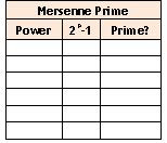
Taking a walk down Geek Lane this week with a look at exploring Prime Numbers in Excel. Specifically, Mersenne Prime Numbers. A Mersenne Number is a number in the form of Mn=(2^n)-1. Although Excel is not robust enough to explore this in depth, it is nonetheless interesting to see what can be done.

So, assuming you have a bit of geek in you, here is what you can do.

1. Create a simple spreadsheet with a similar format to the following starting in A1:

2. Starting in A3, insert consecutive numbers starting with 2 into Column A.
3. In B3, place the formula, “=(2^A3)-1”and copy down with relative references
4. Go to the Blue Moose Technology site (Thanks, Blue Moose!) and copy the prime code into a new module in your workbook
5. Finally, use the resulting “ISPRIME” custom function starting in C3 to determine if the numbers in the B column are prime

Obviously, this exercise is not of interest to everyone, but if you find both Excel and Prime Numbers exciting, give it a try. You might find you are “Ready for Prime Time”.

Microsoft Excel 2010 Technical Preview

Reading and speculating on future versions of Excel (and Microsoft Office in general) can heighten anticipation for what users always hope to be a panacea for all of their work-related challenges. The latest version of Excel is due to be distributed to select users for a Technical Preview this July.

The new application is purported to offer a forward-looking browsing experience and an essentially unprecedented open source interface. There are reportedly many cool new features, including much more powerful Pivot Table tools. This is particularly exciting for anyone doing business analysis in Excel.

Also of note, the new MS suite will be released in both 32 and 64 bit versions, so hardware that can run the current Office 2007 will be able to handle 2010 as well.

If you are interested in learning more or being considered for taking part in the Technical Preview, you can get additional information and register by following the link below:

http://www.office2010themovie.com/

Happy Excelling!

Paste Special is Our Friend

Have you ever copied some cells in a workbook and pasted it elsewhere, and gotten errors in the target location? If you want to copy what you see and have it appear in the new location exactly as it appeared in the source, you probably should give Paste Special a try.

The problem with using ordinary Copy/Paste is that it will duplicate any formulas contained within the data and transfer them to the new location in a relative manner (I know, I know, let’s not get the relatives involved…). Here’s what you do:

1. Select your data, right-click and choose Copy
2. Select your target cell, right-click and choose Paste Special
3. From the Paste Special menu, choose Values and click OK
4. Bamm! What you see is what you get!

The next time you find yourself in a Sticky Situation (“Sticky” and “Paste” get it… ), try using Paste Special. It really is Our Friend!

Removing Duplicates

When it comes to removing unwanted duplicates in a database, users of Excel 2007 have it easy. The following is a best practice to accomplish this useful task:

To get an idea of what you are working with, first, use the Conditional Formatting:

1. Select the key field(s) in the database containing the possible duplicates
2. Go to Conditional Formatting command in the Style group on the Home
3. Choose Highlight Cell Rules / Duplicate Values
4. Choose a Cell Format (bright yellow fill is good for this purpose) and click OK

If you then want to remove the highlighted duplicates you can do so quite simply by:

1. Select the entire database (be careful not to select any self-generating key fields)
2. Go to the Data tab in the Data Tools group and click Remove Duplicates
3. Select all of the columns and click OK
4. A message will pop up telling you how many (if any) values were found and removed

This is a good way (Easy is always good) to help maintain the integrity of your database. Give it a try: Get rid of those Duplicates!

F3: The Magic Key

Well, “Magic Key” might overstating it a bit, but you work with Named Ranges and a lot of Formulas, the F3 key can save you a great deal of work. Here is what it can do for you:

Let’s say that you have named several ranges (an Excel Enthusiasts best practice) in your workbook. When creating a formula, (in this example, we will find the average of a field named, “Sales”), do the following:

1. Type “ =Average( "
2. The hit the F3 key and
3. Choose your Named Range from the dropdown
4. Note that you can use your Down Arrow on your keyboard to select

This shortcut will save you little bits of time that will add up to many hours of work. (Wow! “Magic” …)

Engaging Charts

As any good presenter knows, you must first Engage your audience in order to effectively communicate with them. With Excel 2007, there is no need to settle for tiresome old charts that everyone has seen before (and probably largely ignores).

Customization is now easy, and can take very little time to apply. Follow a few simple steps to create one-of-a-kind engaging charts. For instance, to create a striking pie chart, try the following:

1. Select your table of data and go to Insert/Charts/Pie
2. On the Pie dropdown, choose a 3-D selection
3. Double-click and choose a color scheme from the Design tab
4. Right-click on the pie chart and select Format Data Series
5. On 3-D Format area, play around with the Bevel and Surface Material options

In very little time, you will find that you can create a unique and compelling chart that is sure to get “Ooohs and Ahhhs”. Give some new pie a try – you may find it very tasty!

Pop-Up Documentation Validation

At times a spreadsheet created by another (albeit brilliant Excel practitioner) can be confusing. The Data Validation tool can help make your worksheets more useful to others. Use this tool to simply add a pop-up window displaying documentation whenever the cell is selected.

Excel 2007 users can follow these steps:

1. Select the cell for the pop-up to appear
2. Click the Data tab of the ribbon
3. Select the Data Validation tool and resulting Data Validation dialog box
4. Choose the Input Message tab
5. Check the Show Input Message When Cell is Selected
6. Enter a title for the pop-up window
7. Enter the text of the documentation in the Input Message
8. Click OK

Give a helping hand to your spreadsheet users. Pop-ups can be a good thing!

That Blank Look

Experienced Excel users know that the IF function is a powerful tool when wanting to return certain words based on the parameters you set within the formula. But what if you want the target cell to remain blank if certain conditions are not met?

The answer is so simple, it will make you laugh. You use quotation marks as with text, but just put a space between them.

=IF(A1 > 365,”Data Error!”,” ”)

In our example, the IF function can help maintain data entry integrity. If the value in cell A1 is greater than 365, “Data Error!” is displayed in the cell. If A1 does not exceed the parameter chosen, there is no need for the message, and the cell remains blank.

Sometimes that “Blank Look” is just what you need. (Just don’t try it when your boss is talking to you…).

Concatenation & Email

Having a spreadsheet of employee names is great, but what if you want to use your data for sending emails? Concatenation to the Rescue!

Let’s say you have a list of employees with the First Names in column A and Last Names in column B. Combining them into an email-friendly column of names in a “Last Name, First Name” format is easy. Here’s how:

Assuming your table starts in cell A1, put the following formula in C1:

=B1&", "&A1

This combines the contents of B1 (last name) with a comma, space, and contents of A1 (first name). Drag the formula down to fill Column C, copy, and paste into Outlook. Presto! You have your mailing list!

“Watching the Action”

Keeping an eye on the values of certain Excel cells can be problematical if you are working with a large spreadsheet (or multiple spreadsheets). Solution: “Watch Window” to the rescue!

The Watch Window can display the value of any cell or cells in a viewing pane that can be relocated on your screen. The simple instructions are:

1. Select the Formulas tab on the ribbon
2. Select Watch Window from the Formula Auditing section
3. The Watch Window will appear
4. Click the Add Watch button to specify the cell(s) you wish to monitor

“All along the watchtower…” (Gotta love Dylan…)

MCAS in Excel 2007

Education and certifications are good hedges against being downsized in these recessionary times. Microsoft has a focused recognition program in their office apps which includes an excellent certification for Excel 2007.

Included in the exam are topics covering:
• Creating and manipulating data
• Formatting data and content
• Creating and modifying formulas
• Presenting data visually
• Collaborating on and securing data

You should have had some time with hands-on experience creating business spreadsheets with Microsoft Office Excel 2007, as well as previous versions of Excel. There are also excellent study materials available which are recommended for even more experienced users.

When you pass Microsoft Office Excel 2007 Exam, you complete the requirements for the Microsoft Certified Application Specialist (MCAS) in Excel 2007.

Interested? Click on the following link for more information:

Microsoft Learning

Moving or Copying a Worksheet

This is a simple tip that you will probably find very handy. If you ever find the need to relocate or copy a worksheet into another workbook, this Move is for you! (“Move”, get it…)

To Move or Copy a Worksheet
1. Right-click a tab, then click Move or Copy on the menu
2. In the Move or Copy dialog box, you can:

• To move the worksheet to a spot within its own workbook, select a sheet in the Before sheet box
• To move the worksheet to another open workbook, select the workbook in the To book list and then click OK
• To keep a copy of the worksheet in your source workbook (rather than deleting it and moving it), select the Create a copy box
  
  Moving Day can be a drag, but using this shortcut, it’s walk in the park…
  

Validation with a Named Range

Using a list with the Validation tool in Excel is a useful way of maintaining consistency in a spreadsheet. Combining it with a Named Range can make it more effective!

Let’s say you are using a dropdown box in a cell that refers to a list of employees. For convenience and to assure consistent spelling, you have created the dropdown box using the List feature on Validation.

Rather than having to put up with the hassle of adding/deleting employees from the reference list and then having to adjust the list range, you can simply Name a Range “Employees”, (with sufficient room to add names in the future), and refer to “Employees” in the list box in the Validation dialogue box.

Give it a try. I think you'll like this “Home on the Range”…

Freeze Panes

This is a very simple, but highly useful Excel maneuver. If you have a long list of data and you want to keep the headings on the screen, simply:

1. Click the cell immediately under the row beneath the column headings.
2. Select View/Window/Freeze Panes (Excel 2007)

You can now scroll your data and still see the headings. Cool, eh? (“Cool”, get it)?

Find What You Want Where You Want

If you work with large amounts of data, you probably find yourself in need of searching for specific items in specific regions of your Excel worksheets. The Find function (Ctrl+F) is one of Excel's most frequently used tools for this purpose.

There are times, of course, when you do not want to search All of your data. If you want to narrow your search to a specific range in your worksheet, (a single column, for instance), you can simply select the range you want to search before pressing Ctrl+F. When the search is performed, only the selected range is included in the exploration, and all else is ignored.

Select your range and hold Ctrl+F. Bamm! There’s your data!