Navigating on Excel

Readers of this blog have said they would like to occasionally return to some of the basics, so today we are going to review the topic of navigating in Excel.

Sailing the seas of your Excel worksheets can be chore unless you know a few simple tricks. For instance, if you wish to go to your last entry at the bottom of a list that contains 30 records, scrolling to where you wish to go is simple and effective. When you have a list containing 3,000 records, however, it is a bit tedious.

As is true with so many Cool Moves in Excel, keyboard shortcuts rule when it comes to saving time moving from one location to another on your spreadsheet.

Here are few Cool Moves you can make without ever touching a mouse:

1. Control / Down Arrow: Goes to last cell in column with data

2. Control / Right Arrow: Goes to last cell in row with data

3. Control / End: Goes to last row, column and cell

4. Control / Home: Returns to cell A1

When using your mouse, another way to navigate to the end of your data (whether in a column or row) is to carefully place your pointer on the adjacent border of cell in your range and double-click. For instance, if you wish to navigate to the last cell in a column of data that starts with cell C1, you can select C1 and double-click on the bottom border of the cell.

Want one additional way to navigate when you know the exact address of some remote cell? Simply enter the address (e.g. ET3000) in the Name Box and Bamm; you have beamed directly to that location.

Try a few different ways of navigating on the Excel seas; you can sail to where you want to be in the blink of an eye!

Dynamic Chart Title (Oh, Wow!)

If you are looking for an “Oh, Wow!” feature for your next report containing a chart, the use of a Dynamic Chart Title is for you! By linking the chart title to a value displayed in a specific cell on your worksheet, you can create a very accessible chart that will amaze and delight your users.

As we have discussed before, it is super easy to create a dropdown list using Validation/List. If you have created a table that changes in accordance with the value shown in the dropdown, (e.g. a salesperson’s name), you can in turn create a chart that shows the updated data (e.g. a salesperson’s performance), along with the sales professional’s name in the title.

Here is how you do it:

1. Select the Chart Title
2. Go to the formula bar and type “ = ” and
3. Select the cell to which you want to link (be sure to use an absolute reference)
4. (Note: The final cell reference formula should look something like: “ =Sheet1!$B$2 ”

Oh, Wow! What a great way to add functionality, ease-of-use, and Pizzazz to your reports!

Happy Holidays, All!

When in Rome...

Once in a while, it is good to have a bit of geeky fun. Although of no real practical use, it can be interesting, (once again, in a geeky sort of way), to play around with Roman numerals. For an Excel user, it is particularly interesting to find that the application has a built-in Roman numeral function.

Practicality, of course, can be overrated, and it is readily apparent that Hollywood, Football, and the Olympics have all used Roman numerals on a regular basis. If you also wish to do this sometime in Excel, (I probably wouldn’t recommend it for your next quarterly report to your boss, unless the individual has a really good sense of humor), you can use the Roman function.

For a classic numeral, (other formats are available, but who needs them…), simply enter a value in cell A1 and type, “=Roman(A1)” in cell B1. Hit Enter and Presto, a Roman numeral of the A1 number! Now you will be all set if the NFL needs someone to come up with the name for the next Super Bowl!

Fun with the Spinner Buttons!

Since they control the data that can be entered and are easy-to-use, so-called “Spinner” buttons can be a clever addition to a spreadsheet. To add a spinner in Excel 2003 and in earlier versions of Excel, click the Spinner button on the Forms toolbar, and then draw your spinner on your worksheet. (You can size the Spinner to your liking.) To add a Spinner in Excel 2007, click the Developer tab, click Insert, and then click Spin Button in the Form Controls section.

Now you are all set to have some fun! Right-click on the spinner, and then click Format Control. On the Control tab complete the values as follows (this is a test, ma’am or sir, only a test…):

1. Current value: 1
2. Minimum value: 1
3. Maximum value: 10
4. Incremental value 1
5. Cell link: $C$7 (Note: Any of these values can be of your own choosing.)

Now when you click the Spinner control, cell C7 is be updated according to the parameters you set. If you have created a worksheet where other cell values or results are dependent on the value in C7, your worksheet will update according to the quantity you select with the Spinner.

How cool is that! Make your Excel worksheets look like someone spent hours of programming time on them in just 5 minutes. Give it a try (people will think you are a Star!).

Conditional Formatting Revisited

Good communication is the life blood and Bane of business. This fact could not be truer than in reports and presentations that involve numbers (Financial and Performance reports are notorious examples). Nothing causes the glazing of eyes like a large table of numbers with row after row of monotonous monotone data.

So how do we get our numerical information across to our stakeholders in an efficient and engaging manner? Well, although Charts are obviously very effective, they are not the only method. Conditional Formatting is a very powerful technique that should not be overlooked.

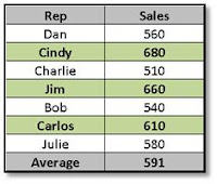
Taking a simple table of sales data as an example, let’s say that you would like to have your audience be able to easily identify those reps with sales greater than the average. First, create a simple formula in the last row that calculates the average of all sales, (e.g. “=Average(B2:8)”). Then set your Conditional Formatting for the first row to highlight (I like to choose my own formatting set to give it a bit of a custom look) if the value in the numerical column is greater than the cell displaying the average (=B2>$B$9).

Then it is a simple matter of selecting the cells with conditional formatting, clicking the Format Painter, and “painting” the rest of your table. Bamm! Instant impact and improved communication! This is Easy (and “Easy” is Good). Give it a try and brace yourself for Accolades…