Option Buttons

In the old Clint Eastwood movie, Magnum Force, Harry Callahan used the line, “A man’s got to know his limitations”.  That may be so, but it is always good to have Options.  For this last post of 2010, I thought it would be interesting to take a look at Option Buttons.

Option Buttons can be very useful in creating Quizzes or Polls in Excel, and are not too difficult to create.  There are a number of steps, but I guarantee that it will be well worth it if you hang in there and give them a try!  Here is how you do it:

1.  Make sure the Developer tab is visible on your toolbar

2.  Under the Developer tab, choose Insert / Option Button (Form Control)

3.  Draw the Option Button box on your worksheet and repeat for however many buttons you wish to have for choices

4.  Now, (this is Important), to make the buttons work together, return to your Insert dropdown and choose Group Box (Form Control)

5.  Then draw your Group Box all the way around your Option Buttons

Stick with me now, we’re almost there!

6.  Right-Click one of the Option Buttons, choose Format Control from the dropdown and select a Cell Link that you want your Option Buttons to populate

7.  Now is where the Fun really begins.  Create a Formula that is based on the value that is shown in the Cell Link

8.  For example, let’s say you have linked three Option Buttons to cell $E$5 and you wanted Option 2 to return a “Correct” response and the others to return “Incorrect”, here is what you do:

In cell E6, type =IF(E5=0,"", IF(E5=3, "Correct!", "Incorrect"))

Now when the user chooses Option 2 of the three possible, they are rewarded with the “Correct” feedback.  Option Buttons, give them a try; “It is always good to have options…”.

Happy New Year All!

            

A Little Excel Magic

Some shortcuts and tips can often appear Magical!  Here are a few of my current favorites:

Select Noncontiguous Cells

If you want to select noncontiguous cells in a worksheet, just hold down the CTRL key and click on the cells you wish to select.  Presto!

Enter Strings Starting with Zero

Sometimes, as in the case with zip codes, you want to enter strings of numbers that start with zero.  To do this, simply type an apostrophe first.  Alacazam!

Rearrange Rows and Columns

So, you have your data are in rows and you want them in columns (or vice versa)?  Highlight the cells that have your data, right-click, copy, and choose Paste Special. Then check the "Transpose" box. Voila!

A Room with a View

Feeling a bit cramped when viewing your spreadsheet?  You can hide columns or rows you don't need to be visible by right-clicking and selecting “Hide”.  Any functions tied to data in the hidden areas will still operate fine.  Open Sesame!

Instant Chart

Impress your friends and family by making an instant chart.  Simply select your data and click F11.  Magic!

I hope you have a Magical (and safe) Holiday Season!

Concatenation Revisited

This is one of my favorite time savers. I teach Excel, and I have had classes as large as 200 students. Since I believe strongly in frequent communication, I keep in touch with individual students and the group as a whole. Having a spreadsheet of student names (or company employees perhaps) is great to stay organized, but what if you want to use your data for sending emails? This is where Concatenation Shines!

Consider that you have a list of students with the First Names in Column A and Last Names in Column B. The good news is that you can easily combine them into an Email-Friendly column of names in a “Last Name, First Name” format is easy. The secret to Concatenation is using Ampersands and cell references combined with quoted text or punctuation. Here’s how to do it:

Assuming your table starts in cell A1, put the following formula in C1 (be sure to note that there is a space after the comma in quotation marks):

=B1&", "&A1

This simple formula combines the contents of B1 (last name)with a comma, space, and contents of A1 (first name). Select C1, place your cursor over the “handle” in the lower-right corner of the cell, and give a quick double-click. This will populate your Column C Email List down as far as you have data in Columns A and B.

Then it is a simple matter of copying the contents of Column C, and pasting into Outlook. Bamm! You have just saved a Ton of Time!

Using the RAND Function

A very interesting and at times very useful function in Excel is the RAND function. This function returns a Random Number that is greater than or equal to 0 and less than 1. Each time your worksheet recalculates, (by reopening or forced recalculation by pressing F9), the RAND function returns a new random number. While some hard core statisticians have voiced concerns about the true Randomness of the RAND function, it suffices for nearly all but the most demanding statistical applications.

The syntax for the Rand function is simply:

RAND( )

If you want to create a random number between two numbers, (where a is the smallest number and b is the largest number), you can use the following:

=RAND()*(b-a)+a

If you want only Whole Numbers you can use:

RANDBETWEEN ()

For example, =RANDBETWEEN(1,200) will produce a random whole number between 1 and 200.

So how can you use this nifty little function? It can be used in myriad ways; for example, it can be used in conjunction with other functions to create a Password Generator. There are countless statistical applications, but you can also use it for entertaining applications. For example, one Excel Enthusiast used it create a Tetris-style game in Excel.

I have used the RAND function in conjunction with other functions and graphics to create a Slot Machine in Excel (send me a request at excelenthusiast@gmail.com if you would like a copy of the Slot Machine spreadsheet).

The RAND function. Great for use in statistical applications, as well as some RANDom FUN!

Choosy Moms Use “Choose”

Having a Choice is (as Martha Stewart would say) “a good thing”. Nested IF functions can be very useful, but they have limitations (the maximum nested functions is 7) and they are cumbersome.

Happily, there is an alternative choice to using these awkward IF functions: The CHOOSE function to the rescue! The Choose function is straightforward and simple to use, plus it can be combined with other Excel features to make it even more powerful! The function returns a value from a list based on a given position (Index Number).

Here is the uncomplicated syntax:

Choose( Index_Number, Value1, Value2, ... Value_n )

Some examples are as follows:

=Choose(3, “Apples”, “Pears”, “Plums”, “Cherries”) returns Plums

It also works with ranges:

=Sum(Choose(2, A1:A20, B1:B20, C1:C20) returns the Sum of B1:B20

You can, of course, link it to the value in a cell, which makes it more flexible. For example, you could link it to A1 which contains the Index_Number.

If A1 contains the number 4, then =Choose(A1, “Apples”, “Pears”, “Plums”, “Cherries”) would return Cherries.

The Choose function can handle up to 29 options, which makes it a great choice in many real-life situations. Give it a try and find out why Choosy Moms Use “Choose”.

Scatterplots and the Coefficient of Determination

One of my favorite charts and accompanying functions are Scatterplot (XY) Chart and the Coefficient of Determination function.

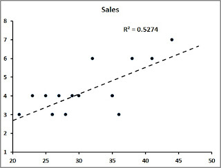
A Scatterplot Chart is commonly used to show the relationship between two variables or sets of data. For example, a sales manager could plot the number of sales calls taken with the number of sales made. Another example is comparing the average length of time a customer service representative takes per call and the overall quality score of their calls.

To determine how strong the correlation is between the sets of data, the wily Excel user can make a Scatterplot Chart and:

1. Right-click on one of the data points and
2. Choose Add Trendline
3. Right-click the Trendline and choose Format Trendline
4. Format the Trendline to your aesthetic preferences and
5. Put a Checkmark next to Display R-squared Value on Chart

The R-squared value is your Coefficient of Determination (COD) that will tell you how strong your data on your two axes. In the graph example above the COD value is .5574 (or approximately 56%) representing a strong correlation (and therefore reliable).

There you have it! Try using a Scatterplot and Coefficient of Determination sometime when seeking the correlation of data sets. It’s easy and can reveal some valuable information.

Happy Thanksgiving All!

Excel Easter Eggs

First of all, I want to congratulate the winner of our “People who use Excel are Cool” Contest that was announced two weeks ago. Gordon Guthrie of Linlithgow, Scotland was the winner with his creation of an Excel clone that works as a native web application. Gordon’s fine work can be viewed using Firefox, Safari or Chrome browsers by accessing the following link:

http://hypernumbers.com

Well, it’s not exactly Easter, but I thought it might be fun to talk about the so-called Easter Eggs that have been hidden in Excel. Virtual Easter Eggs are hidden games or messages that are built into software by crafty developers who have a sense of humor and enjoy building in a bit of intrigue for the “Insiders” who wish to search for the cryptic content. The term was coined in the late 1970s at Atari by the renowned computer game designer, Warren Robinett. Since designers were not given credit for the games they created, Robinett included a hidden screen which said “Created by Warren Robinett”.

The Excel 97 version had a comparatively ambitious Flight Simulator hidden within the application. Using a rather simple combination of keyboard commands brought you to this remarkable simulator.

Although more difficult to access, Excel 2000 included a Car Racing Easter Egg which resembled Spy Hunter.

Excel 2003 included an Office Quiz featuring the Crabby Office Lady. If you still have this version and you are connected to the internet, you can access this egg by typing in “Tortured Soul” in the search box.

Although there are rumors to the contrary, there are no widely-known hidden gems in Excel 2007 or Excel 2010. The general consensus is that Easter Eggs have been eliminated from Excel due to potential security concerns. If you know of any eggs in these versions, please write to me at ExcelEnthusiast@gmail.com. I would love to share them with our merry group! Cheers!

Working with Excel on iPad

Since you are reading this blog on a Kindle, it is likely that you also own (or are thinking about owning) an iPad. Aside from all of the clamor from advocates and naysayers, the iPad can coexist nicely with a Kindle, and can provide an alternative for working on Excel rather than being tied to a full-blown desktop or laptop computer.

There is no doubt that not all Excel’s features are available when working on an iPad. For a great many common tasks, however, it is more than sufficient, and there is something very positive about being flopped on a sofa and still having access to your favorite software. Not only that, but as the software makers further refine and create new applications that can handle spreadsheets, the possibilities continue to grow.

Applications

There are a growing number of applications that the Excel Enthusiast / iPad Owner can use. My favorites are Quickoffice’s Quicksheet and Apple’s Numbers. Although DocsToGo is a worthy contender, most users (in my humble opinion) will find the features and user interface more pleasing with the other two apps. I have been using all three applications since shortly after the iPad’s debut and I find I seldom use DocsToGo for anything other than PowerPoint.

Compatibility

While either Quicksheet or Numbers can handle a great variety of formulas, creating Charts in Apple’s Numbers is a real treat. Both of these applications can import and export in Excel format. This is of keen importance, of course, as what good is a spreadsheet if you can’t export it back to Excel.

Navigating/Viewing

Although it may be a bit foreign at first, tapping to select cells and using the convenient selection handles to choose a range becomes second-nature quite quickly. The now commonly known pinching gestures zoom you in or out on your data and charts, and it is easy to get hooked on these new ways of getting around a spreadsheet.

Sharing

Once you have created your spreadsheet masterpiece on your iPad tool, you can easily email it in its original Apple format, a PDF or, of course, as an Excel document.

Although some will deride this new way of interfacing with your data, I firmly believe that if you give it a chance, you will find that it makes a pleasant and productive alternative way of working with your Excel creations. Cheers!

Contest!

People who use Excel are Cool! They have used Excel for notonly ingenious ways to crunch data and design stunning charts, but also suchthings as tracking weight loss and designing quilts.

They have used Excel in so many unique and interesting ways that I thought it would be fun to hold a contest for the Kindle Excel Enthusiasts subscribers. I am very sure many of you have used Excel in ways that be of great interest toother Excel Enthusiasts.

So, here are the simple rules:

1. Send an email to excelenthusiast@gmail.com

with a brief description of the cool and/or innovative way you have used Excel.

2. Attach an example if you wish, and please keep the attachment to less than 3mb.

3. Get your entry in by midnight November 15.

The winner will receive a new 8GB Kingston Datatraveler flash drive via U.S. mail the following week, and will have their name and Excel creation announced in the following week’s blog along with any honorable mentions.

Please let me hear from you; it will be Fun!

Four Fun Ways to Liven Up Your Excel

Here are Four Fun Ways to spiff up your Excel workbooks and worksheets (sure to amaze your colleagues!).

1. Change the Color of Your Sheet Tabs

Right click on your worksheet and select “Tab color” option to change the worksheet tab color.

2.  Insert a Quick Organization Chart

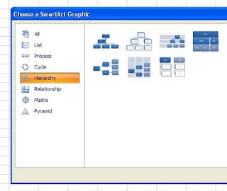
Clickon the Insert tab on the toolbar and go to SmartArt and choose the “Hierarchy”group.  Pick the Org Chart that suits your fancy.

3.  Hide the Grid Lines on Your Worksheets

Do away with clutter by going to the View tab on the toolbar and Deselecting the box next to Gridlines.

4.  Add a Rounded Border to Your Charts

Simply right-click on your chart, select Format Chart option, and choose “Rounded Borders”.

There you have it!  Four really Fun Ways you can liven up your Excel workbooks and look Very Cool doing it!

This Week's Post

Greetings Excel Enthusiasts!

Just a note to say that some of you may find this week's post on the Frequency Function a bit intimidating, but hang in there, its worth a try!

I am also serious about lending a hand on a real-life project if you need any assistance.


All the best,

Bob

rdelamartre@gmail.com

Using the Frequency Function

Whether you are in the corporate or academic world, there are times when you want to know investigate how frequent values within particular ranges occur. An excellent solution in Excel is the Frequency Function.

This unique tool works as an Array function that counts the number of values that occur in each specified interval for a given set of values and a given set of intervals (or “Bins”, as they are often referred).

The FREQUENCY Function syntax is as follows:

 FREQUENCY(data_array, bins_array)

The function is entered as an Array formula after you select a range of adjacent cells (C2:C5 in our example) into which you want the distribution to appear. After you select the data and bins arrays, press CONTROL+SHIFT+ENTER.

Please Note: The number of elements in the returned array is one more than the number of elements in bins array. The extra element in the returned array returns the count of any values above the highest interval.

Example:

Formula Description and Result

=FREQUENCY(A2:A10,B2:B4)

1. Number of scores less than or equal to 75 (4)
2. Number of scores in the bin 76-84 (2)
3. Number of scores in the bin 85-94 (1)
4. Number of scores greater than or equal to 95 (2)

The Frequency Function can be a great boon to you regardless of the type of industry you work in.

Important Reminder: Be sure to Select your Entire Range (once again, C2:C5 in our example) where you want your results, and then enter the formula with the Array Keyboard Combination of CONTROL+SHIFT+ENTER.

Please send me an Email at rdelamartre@gmail.com if you have any problems setting up your table.

Happy Excelling All!

Customizing Excel

There is no doubt that the Standard, Off-the-Rack Excel Setup is just fine for most folks. It provides the features and does what most people want it to do. Since you are a reader of the blog, however, you do not fit into the mainstream of Excel users.

Excel offers a plethora of choices in customization for the uncommon user. Excel 2007, for instance, offers a One-Stop-Shopping location to choose a vast array of Excel Options. This Swiss Army Knife location can be found by going to the Office Button, and clicking on the Excel Options button in the lower right corner.

From there, you will be presented with the following General Categories of options:

1. Popular
2. Formulas
3. Proofing
4. Save
5. Advanced
6. Customize
7. Add-Ins
8. Trust Center
9. Resources

For example, two of my favorite options, the Analysis ToolPak, and Microsoft Solver can be found and activated by going to the Add-Ins category. Another common favorite is setting the default font and font size from the Popular category. Yet another favorite, found in the Save grouping, is adjusting how often Excel automatically saves your information.

Customizing Excel can provide nearly endless benefits for the uncommon user. If you haven’t already done so, check them out (You’ll be the envy of all of the other Excel Users on your block…).

AutoFill with Week Days

Let’s say that you are working on a project where you want a list of weekdays, but you don’t want to manually enter them in your column or row. What is the solution? Autofill to the Rescue!

Autofill is, of course, a common and highly useful tool that most any regular Excel user is familiar with. You may not have noticed, however, that you can also use this tool for Autofilling Weekdays.

Here’s How You Do This:

• Enter the starting day into a cell (Monday, Tuesday, whatever…)

• Place you mouse pointer over the lower-right corner of the cell (the small black square is the “handle”) until you see the narrow crosshairs appear

• Right-click the handle and drag to select the range you want to fill with weekdays

• When you release the mouse button, a dropdown menu will appear

• Select Fill Weekdays

Voila! A filled series of Weekdays! This tip works in Excel 2010 as well as earlier versions, so give it a try some time!

Hide and Seek

“Keeping Things Simple” is almost always a good thing. Hiding a worksheet is one way of keeping your workbook tidy, and also can serve to protect sensitive data from prying eyes. As with all things Microsoft, there is more than one way to hide and unhide a worksheet in an Excel, but we are going to look at the most straightforward method of doing this in Excel 2007 and 2010.

To hide a single worksheet in Excel, open the worksheet and then simply Right-Click the tab and choose Hide. To Unhide it, simply right-click any tab and choose the worksheet to Unhide from the dropdown list.

To hide multiple worksheets, just select the first worksheet to hide with your mouse, hold down on the Ctrl button on your keyboard, choose the tabs of other worksheets to hide, and then right-click and Hide.

Please note that if you want to Hide a worksheet so no one else can Unhide it, simply Protect your workbook with a password by going to Review ribbon on the toolbar ribbon and choose Protect Sheet in the Changes grouping.

Easy and effective; always a good combination. Give it a try, and keep things simple and private. Happy Exceling!

MATCH and INDEX = POWER!

You say you like using the VLOOKUP function, but would like something a bit more versatile and powerful? Look no further than the MATCH and INDEX functions!

MATCH returns the row number of the location in an array of value you specify. Using the example above, the number “4” is returned by the formula:

=MATCH("Sacramento", $A$2:$A$6,0)

INDEX returns the value that you identify by row number in an array. Using the example above, “Sacramento” is retuned by the formula:

=INDEX($A$2:$A$6,4)

Using the INDEX and MATCH functions In Combination, we can set up a code retriever as shown in cells E1:F2, by inserting the following formula in cell F2 (This will return "126"):

=INDEX($C$2:$C$6,MATCH(E2,$A$2:$A$6,0)) 

Using MATCH and INDEX functions together, now that’s POWER!

Three Ifs

“If” functions can really help you make sense of your data. Here are my three favorites:

COUNTIF: =Countif(Range, Criteria)
For the Criteria, you can specify a cell, a simple number such as 10, or use a greater-than or less-than criteria such as “>20”. Be sure to use the quotation marks if doing a great-than or less-than analysis.

SUMIF: =Sumif(Range, Criteria, SumRange)
The Criteria is the same as in Countif, but you have the option of applying it to a “SumRange”. These are the actual cells to add if the cells in the Range match the criteria. If SumRange is omitted, the cells in Range are evaluated by criteria and added accordingly.

IF: =If(Condition, Value If True, Value If False)
This function is extremely valuable as a stand-alone or in conjunction with other “nested” functions. You can use cell references for the “Value If True” or the “Value If False”, or insert words (e.g. If(A1>10, “Pass”, “Fail”). Just be sure to use quotation marks if inserting actual words.

There you have it! Three terrific “If” functions. Give them a try some time IF you have a chance!

Scrolling, Scrolling, Scrolling!

If you have a spreadsheet that needs incremental updates of the numbers in certain cells, clicking on the cells and typing in the subsequent number can be tedious. Using a Scroll Bar can make it considerably easier to increase (or decrease) a value, such as a number, time, or date by allowing you to Scroll through a range of values when you click the scroll arrows or when you drag the scroll box. Besides that, it makes your Excel worksheet look very cool!

Here is how you do it on Excel 2007 and 2010:

1. Choose the Developer tab and go to Insert on the Controls grouping
2. Click the Scroll Bar under the Forms Controls section
3. Draw the bar next to the cell you want it to control (it can be either vertical or horizontal)
4. Right-click on your new Scroll Bar and choose Format Control
5. Select the Control tab on the Form Control and choose your own custom parameters
6. Insert the cell reference in the Cell link (e.g. $A$1)

Here is how you do it on Excel 2003 and Earlier Versions:

1. Go to the Forms toolbar and click the Scroll Bar
2. Draw the bar next to the cell you want it to control (it can be either vertical or horizontal)
3. Right-click on your new Scroll Bar and choose Format Control
4. Select the Control tab on the Form Control and choose your own custom parameters
5. Insert the cell reference in the Cell link (e.g. $A$1)

Bamm! There you have it! Not only will this save you tedium, it will make you look like the Excel Rock Star that you are!

Double-Click is Our Friend!

Double-clicking is a powerful tool that can save you many hours of work. Try any or all of the following six techniques and see if you do not agree that “Double-Click is Our Friend!”


1. Autofit Column Widths by Selecting Multiple Columns and Double-Clicking Between the Headers
A relatively common, but highly useful move!

2. Double-Click on the Office Button to Close Excel
Works great in Excel 2007! Displays “Do you want to save…” if the workbook is not saved.

3. Auto-Fill a Series of Cells with Data or Formulas by Just Double-Clicking
Just select the formula in first cell, double-click in the “handle” (small black square in bottom-right-corner) and Presto! This works for formulas, auto-fills (of numbers, dates, etc) as long as the adjacent column has data.

4. Double-Click on Ribbon Menu Items to Collapse Ribbon to Get More Space
Another cool Excel 2007 feature. Enables you to collapse the ribbon to one line.


5. Lock Format Painter and Reuse it with Double-Click
Double-clicking the Format Painter locks the format so you can use it repeatedly in your worksheet – Awesome!

6. Jump to Last Row or Column in Table with Double-Click
This is my favorite. Just select any cell in the table and double click on the cell-border in the direction you want to go. Speedy!

There you have it!  Try these simple techniques out and find out why “Double-Click is Our Friend!”

More Cool Excel Shortcuts

Back in April, I posted my own personal Top Ten Best Excel Shortcuts in reverse order (ala Letterman’s Top Ten…). Here is an additional List of Five of my favorite shortcuts for use with Named Ranges:

5. Name a Range
Select the range, and then click in the Name Box (far left on the formula bar) and type a one-word name

4. Quickly Name All of Your Ranges
Highlight your entire database including the headings with Ctrl + A and then click Ctrl + Shift + F3

3. Go to a Named Range
Click F5 (Great for selecting Named Ranges!)

2. Edit a Named Range
To delete or edit a named range click Ctrl+F3.

And the Number One Best Named Range Shortcut Is (Trumpets, please)...

1. Display the Paste Names Dialog Box for Use in Formulas
Click F3 and use your arrow keypad to select (Super helpful when creating long formulas)

Working with Named Ranges Rocks – Use these tools to make your Excel life easier!

Spiff Your List with Conditional Formatting Icons

Many of us use Excel to keep Lists of Stuff. It may be as simple as a grocery list or as complex as a due-diligence list for a corporate merger. Starting with Excel 2007, you can use sets of Well-Formatted Icons with your lists (and replace lists using the drab “x”).

For an example, let’s suppose we are organizing a Lutefisk Promotion Event in Minnesota, (I’m originally from Minnesota, doncha know – Oh yeah…), and you want to Spiff Up your checklist that will track who will attend.

Here is how you do it:

1) Select the range of cells in which the checkmarks will appear (from C3 to C8 in our example) and put a number 1 in each cell where you want a checkmark
2) Click Conditional Formatting on the Home tab, choose Icon Sets and pick the set that includes the Green Checkmark
3) Go back to Conditional Formatting and choose Manage Rules
4) Click Edit Rule and put a check in the Show Icon Only box and Apply

That is It! Your lists will instantly take on new character and professionalism (and it wasn’t even hard, doncha know…)

Indirect and Validation

Interactive reports are powerful tools that can provide the user with multiple sets of information in a One-Stop, Professional Format. There are many ways to create reports of this type, (background pivot tables, Boolean functions, etc), but one of the easiest is to make use of the functionality in Validation combined with the Indirect Function.

Although there are many uses for the Indirect Function, used in its simplest form it will take the Word in the cell it is referring to and return the Named Range.
Using the small spreadsheet in the graphic above, try the following:

1) Create your Named Ranges by selecting each of your ranges and typing the new Name in the Name Box on the upper-left corner of your worksheet. In the above example graphic, name each of the monthly rows (excluding the cells with the month name) for the four units. For instance, for August, select C12:F12 and name it August.

2) To get a convenient Dropdown Box, go to Data Validation in Tools and choose Allow List (you can choose the list of items that you want to appear in the dropdown box). For example, in the above graphic, the cell C2 with “April” in it contains the interactive dropdown created using the list of months.

3) Now the fun begins! In cell D2 insert the formula “=SUM(INDIRECT(C2))”. The Indirect Function reads the name of the month you choose with the dropdown box in C2 and the formula sums up the total for the four units.

Try this straightforward, easy way to make an interactive report. They’ll soon put up statues in your honor!

Troubleshooting Formulas

Let’s face it, problems happen in Excel. One of the most common issues, of course, involves the use of formulas. The problem is that (this is particularly true if you were not the original creator of the workbook and have “inherited” it) that you may not know which cells have formulas and which are simply data.

An easy way to identify the cells with formulas and display them is to hold down the Ctrl button and press ~. When you press this keyboard combination, all of your formulas will appear in their cells (pressing the combination again will bring back your original view).

Another vexing problem can be determining exactly where a formula is drawing its information from. Excel contains a nifty (do people still say “nifty”) tool for clicking on the formula cell and tracing its Precedents. For Excel 2003, go to Tools / Formula Auditing. For Excel 2007, go to Formulas / Formula Auditing.


Clicking on Trace Precedents will give you a Graphical Layout with Arrows and Worksheet representations showing you from where your information is being derived.

Ctrl + ~ and Trace Precedents; two excellent tools to help you get your Excel workbook back on track.

DateDif Revisited

A little over a year ago, I discussed the obscure DateDif function, and it was a readers’ favorite.

As I mentioned in my 2009 post, Microsoft has for reasons only they know, mysteriously chosen not to include documented information of this fascinating function in Excel. DateDif is a very useful (I think it is essential) tool for doing calculations with dates. Here is a refresher with some additional good information.

The syntax of the function is as follows:

=DateDif(First Date, Second Date, Time Interval)

Where the Time Interval is expressed as follows:

d   (Days) = Number of days between the dates
m  (Months) = Complete calendar months between the dates
y   (Years) = Complete calendar years between the dates

Note: The Second Date must be greater than the First Date, or you will get a Number Error.

An entertaining application of this function is to nest the NOW() function into it and calculate a person’s age as follows (Note: the “BirthDate” can refer to an easily changed cell value):

=DateDif(BirthDate, NOW(), “y”)

Special Note: If you put the Time Interval in the function directly, be sure to put “quotation marks” around it (e.g. “m”). If you put it into the formula via a cell reference, do not use the quotation marks (e.g. the cell should contain m, not “m”).

There are a great many ways to use the DateDif function, so give it a try some time. You may wonder how you ever lived without it!

Dynamic Named Ranges

Nearly two years ago, (see my September 15, 2008 post), I wrote about the wisdom of using Named Ranges in Excel. Using a Named Range in a formula does away with the need to make the range an absolute reference because it will always point to the correct range, regardless of where you copy the formula.

The only problem with a Named Range is that if you have a static cell reference, (e.g. $A$1:$A$20), when you add additional data, you will typically need to go to the Name Manager and Change the reference. What a drag!

Happily, there is an easy solution. Excel allows you to enter a Formula in the Named Range reference. Although there are several formulas that work for this purpose, the following one is one of the most versatile. Let’s suppose that you have you data in Column B, and you do not want to include the header in B1. By using this formula, and assuming you do not have any blank cells, (which is a bad database management practice anyway…), you will include your entire range on a Dynamic basis:

=INDIRECT(CONCATENATE("$B$2:$B$", COUNTA($B:$B)))

As a consequence, more data can be added to your database, and your Named Ranges will always remain Up-to-Date with no muss, no fuss. Wow, that Rocks!

Importing Problem? Change Text to Numbers!

Many of us have occasions where we are importing files that were not created in Excel. Usually this causes no problems, but once in a while when you import from other sources, your numeric values may appear to be numbers, but they act like text!

Happily, this is easily solved by converting the values into numbers. To resolve this problem, simply do the following:

1. Click a blank cell in the worksheet, and Type the Number 1 in the cell

2. Right-click, (“Right-click is Our Friend”), and Copy the cell with the number 1 in it

3. Select the range that contains the values you are converting to numbers

4. Right-click and choose Paste Special

5. On the Paste Special menu, click Multiply, and then click OK

So how do you know if you have been successful? Well, you can set up a simple function to see if the values now act as numbers, or you can check out the alignment of the numbers in the cells. If you are using a common format, the numbers will be aligned on the right and the text values will be aligned on the left.

Importing from a source other than Excel? Keep this little trick in mind, and Easily Convert your Values to Numbers! Rock On!

Rock and Roll with Your Ctrl Key!

This week discussion is on Three Cool Things you can do with your Ctrl Key:

#1 - You can make Noncontiguous Selections of cells. Now that’s just a fancy-shmancy way of saying you can select any cells you want, regardless of whether they are next to each other in a column or row. Simply hold the Ctrl key while you click any single cells or select any range of cells.

Bonus: You can also use the AutoCalculate tool at the bottom of you worksheet to analyze any combination of individual cells you have selected by holding down on the Ctrl key.

#2 – Using the Ctrl key enables Fast Navigation. By holding the Ctrl key and any Arrow Key, (up, down, left, or right), you can Instantly Transport to the last populated cell in that direction.

Bonus: Hold down the Shift key while you click any Ctrl-Arrow Key combination to Select All the cells between where you are and where you are transporting to (“Beam me up, Scotty…”)

#3 – You can also use the Ctrl key to Speed Up Data Entry. Let’s say that you want to put the same number, same string of text, or formula into a series of cells. You could do it the slow way by typing the number, string, or formula into the first cell and then copying and pasting it into the destination cells. But by select all of the cells you want to populate, typing the entry, and then pressing Ctrl Enter (be sure not to merely hit Enter), All of Your Selected Cells will be Identically Populated Instantly!

Now, I ask you, Does that Rock or What?

Funky Histogram Anti-Chart

Charts are tremendous tools that visually represent the often dry data that is contained in a table or database. Sometimes it can be a hassle to create one using Excel standard chart-building tools, especially if you want something basic (but still dynamic).

Here is a way to create a Funky Histogram-Style Chart by employing the little-used REPT function. This function repeats a text string the number of times you specify. For instance, the following formulas returns seven dollar signs: =REPT(“$”, 7)

One nice aspect of this simple technique is that it works in Any Excel Version. (Something that can’t be said about the Data Bars feature in versions 2007 and 2003.)

Let’s say that you have a table with Months in Column A, Sales in Column B, and we want our Histogram Chart (let’s call it an Anti-Chart, since we are not using Excel’s typical charting capabilities). We can then insert the following function in our Chart Column D: =REPT(“$”, B2/1,000).

The reason we are dividing the number in B2 by one thousand is to keep the scale of the resulting Anti-Chart to a reasonable width. Simply enter the formula into cell D2 and drag it down to complete your visual illustration of your data. Bamm! Anti-Chart!

Camera Tool – Just Say Cheese!

A picture may be “worth as thousand words”, but sometimes a graphical representation of a chart can use a little support from the source table with the numbers. With the Camera Tool, you can have the Best of Both Worlds.

Though initially hidden on Excel, the Camera Tool can be highly useful when you are presenting a chart and would like to include a resizable image of the source data included within your exhibit.

To find it in Excel 2007, simply right-click your toolbar and choose “Commands Not in the Ribbon”. Then scroll down to Camera and click Add.

To find it in Excel 2003, right-click the toolbar and choose "Customize" / "Commands" and choose "Tools". Then scroll down to the Camera and drag it onto your toolbar.

After that, it is easy (and it hasn’t even been hard…):

1) Select the data table of which you wish to "take a picture" and Click the Camera Icon on your toolbar
2) Then, go to the area on the sheet on which you want the data to appear, and Left-Click
3) Bamm! You have an image of the table (Resize and Reposition if desired).

Bonus! This “image” of your source table is Linked to the original table. Any change you make in the original table will be reflected in the new table you have placed on your chart.

Now, I ask you, is that cool or what! Cheers.

Working with the DATE Function

Working with dates in Microsoft Excel can be a puzzling and, at times, aggravating experience. Adding days, months, or years to a date can be at first a mystifying task.

Happily there are some excellent time functions built into Excel, and one of the most versatile is the (cleverly named) “DATE” function.

The syntax of the DATE function is =DATE(Year, Month, Day), therefore if you enter as follows, =DATE(2010, 6, 17), it will return today’s date of June 17, 2010.

What is particularly Cool about the DATE function is that it very flexibly accepts inputs from cells, functions, and calculations. For example, =DATE(2010+1, 6, 17) returns June 17, 2011. =DATE(2010, 6, 17+7) returns June 24, 2010. You get the picture.

The DATE function can handle more complex situations as well. For instance, =DATE(2010, 6+9, 17) returns March 17, 2011 (Hey, isn’t that St. Patrick’s Day?...).

So let’s say that you have an interactive What If report that has cell B1 with a continuously updated current date, (you can use the =TODAY() function for that), and cell C1 displaying the date which is a variable of numbers of years in the future based on the value you place in cell A1. Your formula in C1 would look like the following:

=DATE(YEAR(B1) + A1, MONTH(B1), DAY(B1))

If today is June 17, 2010 and you have the number 4 in cell A1, the above formula would return June 17, 2014.

Take a few minutes and experiment with the DATE function. It is one “date” that will never disappoint.

First Names and Last Names

As Excel practitioners, we are frequently presented with data that is Not in an ideal format. For instance, let’s say you are presented with list of employee names showing the Entire first and last name in each cell in a column.

As any good database manager knows, it is best to Break Down or Parse Your Information into the smallest discreet portions reasonable. To facilitate maximum information retrieval, you would naturally prefer to have the first names in one column and the last names in another column. If you have hundreds of employees in your company this would, obviously, be Pure Drudgery to convert manually.

Extracting the first names and last names into their own separate fields (columns) with Convenient Excel Formulas is a Breeze. Here is how you do it.

The Excel functions that we will be using in the formulas are:
LEN - Returns the number of characters in a text string
FIND – Returns the starting position of one text string within another text string
LEFT – Returns the specified number of characters from the start of a text string
RIGHT - Returns the specified number of characters from the end of a text string

Okay, here we go! To extract just the First Name, use the following formula:

=LEFT(A1, FIND(" ", A1, 1)-1)

To extract just the Last Name:

=RIGHT(A1, LEN(A1)-FIND(" ", A1))

These relatively simple formulas can really save your day sometime. Go ahead, give them a try!