Reverse Conditional Formatting

Here is a Very Interesting Trick that you probably have never run across. I think we can all agree that it is almost always helpful to have Visual Cues in Excel, and this one takes an Unusual Approach.

Let’s say you have a worksheet in which you are entering data in a column, and you want it to be Obvious if a cell within that column is Blank (a Best Practice for proper database maintenance). Here is a unique way to do this:

Let’s assume you are going to be putting data in the short range of A1:A10.

1. Your first step is to apply a Fill Color to your range (in this case, A1:A10)

2. Then select your range and go to Conditional Formatting / New Formatting Rule

3. Choose Use a formula to determine which cells to format and put the following:

4. =IF(NOT(A1=""), TRUE, FALSE)

5. Finally, for your Format, use Fill / No Color

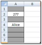
Now whenever you place data (numbers, text, or mixed) in one of your cells in the range, the Fill Color is Cleared! How Cool is That!

Whenever you have a cell that has NOT had data entered into it, the original Fill Color remains. Give it a try; I think you will find this to be another Great Trick in Your Excel Tool Belt!

The Beat Goes On…

Since you are reading this blog, it may be likely that you have influence within your company as regards the software they adopt.  When it comes to Excel, a recent survey showed that many companies still use Excel 2003, some use Excel 2007, and a comparative few have adopted Excel 2010.

Once again, since you are a reader of this blog, you are probably and Early Adapter, and would like to see your company update to the latest version of Excel.  To that end, I have condensed the most compelling reasons to update:

Reason to Upgrade from Excel 2003 to Excel 2007

• More Room:  15 times more rows and 62 times more columns

• Pivot Tables:  Many enhanced pivot table features

• Versatile Functions/Formulas:  Over 8 times the number of arguments and length

• XML Formats:  Better integration with back-end systems

• Dashboards:  Easily created to track key indicators

 Reasons to upgrade from Excel 2007 to 2010

• Recording Chart Macros:  Now available in Excel 2010

• Sparklines:  Great new mini-charts that can enhance understanding of data

• Statistical Functions:  Financial and math functions, as well as the wizard have been much improved.

• Conditional Formatting:  Engaging and intuitive new formatting now available in Excel 2010

• Improved Productivity:  The company’s  Excel Gurus can leverage the enhanced features

Like so many other things in our increasingly technological world, if you don’t keep up on a regular basis, you can one day find yourself being passed by at the parade of progress.

Counts!

Now, some people have said that I am a bit “Batty”, but that’s another story. As we explored two years ago in this blog, there are several ways to Count (Count/Dracula/Bats, get it?...) your data in Excel.

It is important to know the uses and differences of the major types of Count Functions. In summary, they are:

1. COUNT: Simply counts the number of cells in a range that contain a number

2. COUNTA: Counts the number of non-blank cells in a range (including those with text)

3. COUNTBLANK: Counts the number of empty cells

4. COUNTIF: Flexible counting function (this can be a little tricky, so we will explore with some examples)

The COUNTIF function can be challenging to some users because of the prevalent use of quotation marks within the formulas. The following examples will demonstrate how it works (in each case, the formula uses a range named Data):

Count the number of cells that contain the word "James" (not case sensitive):
=COUNTIF(Data,"James")

Count the number of cells that contain the words "James" and “Suzanne”:
=COUNTIF(Data,"James") + COUNTIF(Data,"Suzanne")

Count the number of cells containing any text (ignoring the numbers):
=COUNTIF(Data,"*") Count the number of 3-letter words: =COUNTIF(Data,"???")

Count the number of cells containing text that begins with the letter "T":
=COUNTIF(Data, “T*”)

Count the number of cells that contain a value greater than or equal to 15:
=COUNTIF(Data,">=15")

Count the number of cells that contain a value from 5 to 20:
=COUNTIF(Data,">=5")-COUNTIF(data,">20")

This is, I might add, not the best tool to use in many cases. It does, however, come in handy frequently when you analysis requirements are not too demanding. I hope you have had a good week so far, and that you make your weekend, Count…

~ All the best ~

Troubleshooting Excel

Have you ever Inherited an Excel workbook that simply didn’t make sense? As we discussed in this blog a couple of years ago, problems inevitably happen in Excel. One of the most common issues is, of course, the use of formulas (and, let’s face it, the peculiar way some users set up his or her workbooks).

Troubleshooting is, without question, a Valuable Skill in Excel!

An easy way to identify the cells with formulas (and display them) is to hold down the Ctrl button and press ~. When you press this keyboard combination, all of your formulas will appear in their cells (pressing the combination again will bring back your original view). That is a good start for determining what is going on “behind the scenes”.

Of course the foregoing does not solve all of your investigative challenges. The Vexing Problem can be trying to determine from where a formula is drawing its information. Excel contains an Elegant Tool for clicking on the formula cell and tracing its Precedents. For Excel 2003, go to Tools / Formula Auditing. For Excel 2007 and 2010, go to Formulas / Formula Auditing.

Clicking on Trace Precedents will give you a Graphical Illustration with Arrows that show you from where your information is being derived.

Ctrl + ~ and Trace Precedents are two excellent tools that can help you figure out those cryptic Excel workbooks that you inherit from others. Such a good thing…

Add a Watermark!

There are times when an Excel user may want to include a WATERMARK to indicate a Special Status of an Excel worksheet. You may wish to mark it CONFIDENTIAL or DRAFT, and a watermark can be an ideal solution.

Although this functionality is not built-in to Excel, it is not difficult to place a Picture in your Header to mimic this effect with a few brief steps:

1. Using WordArt, you can easily create an image (such as CONFIDENTIAL) and then upload it into Paint (or other image-handling app) and save it as a .png file.

2. Open the worksheet in which you wish to display your watermark

3. Click on Header & Footer on the Insert tab ribbon

4. Click on Picture on Design tab ribbon and choose your watermark picture

5. Resize your watermark picture by clicking on Format Picture dialog box, select the Options that you want on the Size tab.

It may take a few minutes to do this the first time, but the results are really quite effective. If you ever need a Watermark in your Excel worksheet, give it a try!

Playing Catch-up?

Some of us work for companies that have been a bit slow in adopting newer versions of Excel. Considering the state of the economy these past few years, this is understandable. The fact is, according to a couple of studies, some companies are just now adopting Excel 2007 for their employees.

The change from Excel 2003 to 2007 has been, and is, challenging to many Excel users. If you or someone you know is working through the Learning Curve of transitioning to Excel 2007, there is a nifty little Add-in available from Microsoft that can get a user up-to-speed in very little time.

As Microsoft states on their website, “This add-in adds a Get Started tab to the Excel 2007 Ribbon. Commands on this tab give you easy access to free content on Office Online, such as training courses, video demos, and other Office Online content designed to help you learn Excel 2007 quickly.”

To get this handy little Add-in, you can go to the Microsoft Add-ins site and follow the easy installation instructions: http://office.microsoft.com/en-us/downloads/CD010214099.aspx

Anything that can make a user’s life a little easier is, in the words of Martha Stewart, “A good thing”. Cheers!

What’s Happening NOW?

There are a number of Really Cool ways to use the Time and Date functions in Excel that are both effective and Fun! Let’s take a quick look at them:

The NOW function positions the Current Date and Time into your spreadsheet. Simply enter =NOW() into any cell, and Excel displays the Date and Time in your worksheet. If you want to limit it to just the Date, use the TODAY function, =TODAY().

Using either of the methods above will insert information that will be updated Every Time You Open the Workbook. But what if you want to enter a Static Date that does not update? That would be a Great Way to Date Stamp your work wouldn’t it?

Well, you are in luck! Just select a cell and hold down the Ctrl key and press the Semicolon ( ; ) on your keyboard. Bamm! Instant Time Stamp!

This is one of those Tricks that can be a practical boon to your Excel Life. Have Fun!