Reverse Conditional Formatting

Here is a Very Interesting Trick that you probably have never run across. I think we can all agree that it is almost always helpful to have Visual Cues in Excel, and this one takes an Unusual Approach.

Let’s say you have a worksheet in which you are entering data in a column, and you want it to be Obvious if a cell within that column is Blank (a Best Practice for proper database maintenance). Here is a unique way to do this:

Let’s assume you are going to be putting data in the short range of A1:A10.

1. Your first step is to apply a Fill Color to your range (in this case, A1:A10)

2. Then select your range and go to Conditional Formatting / New Formatting Rule

3. Choose Use a formula to determine which cells to format and put the following:

4. =IF(NOT(A1=""), TRUE, FALSE)

5. Finally, for your Format, use Fill / No Color

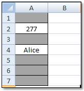
Now whenever you place data (numbers, text, or mixed) in one of your cells in the range, the Fill Color is Cleared! How Cool is That!

Whenever you have a cell that has NOT had data entered into it, the original Fill Color remains. Give it a try; I think you will find this to be another Great Trick in Your Excel Tool Belt!