Intersections

The Intersect Operator is yet another somewhat obscure, but highly useful Excel tools.  Many of the ways to glean information from Excel tables involve cumbersome formulas that can take an Excel guru a considerable amount of time out of his or her busy day.  The Intersect Operator, is not only Powerful and Versatile, it is also quite Simple to use!

The function of this handy tool is to use the vertical and horizontal ranges in a cross-tab Table or Database, and find the value at the Intersection (ergo, the Intersect Operator…).  The syntax (Special Note: Be sure to use No brackets or commas…) is simply:

= (RangeName1 RangeName2)

For the Ranges, you can use the generic names such as =(C2:C42 A10:K10).  Whereas this gets the job done and may be advantageous in limited circumstances, using Named Ranges is much more effective.

As a reminder, you can very quickly name all of the ranges in your database by selecting all cells (use Ctrl + A), and the click Ctrl + Shift + F3. This will bring up the Create Names dialogue box as shown below.  Just click OK, and Bamm!  Named Ranges!

Once you have your ranges Named, you can then (as with the example below where we are finding the 3^rd Quarter Sales for Los Angeles) find a value with the modest function (in Cell E5 in our example):

=(Los_Angeles Quarter3)  Note: Be sure to include the space between the column title and the row title.

 

There are, of course, other ways of obtaining this information in Excel, but the Intersect Operator is certainly a worthy addition to any Excel user’s tool belt.

New Excel Features on iPad

Back in April we talked about the advent of Excel, (along with Word and PowerPoint), on iPad.  For those of us who have become heavily dependent on iPads, this was great news!

As with any software product there is, of course, room for improvement.  Many of us submitted suggestions for Additional Features and Tools for this convenient addition to our Excel capabilities, and as of a few days ago, Microsoft has come out with the new Excel 1.1 for iPad.

So, what is new in Excel for iPads?  Here are some of what I consider to be the Best of the Best:

·        Flick to Select: This is remarkably easy and very handy.  Simply flick a cell’s selection handle in any direction to quickly select all the data in a row or column.  Very cool!

·        Use an External Keyboard:  Although I am not a big fan of using an external keyboard with an iPad, (it is a tablet, after all…), it is sometimes useful to do so.  Now you use the same keys to input data and move around a worksheet just as you would on your PC or Mac.  Good stuff!

·        Send Files as PDFs: You can now send Excel files as PDFs. 

·        More Printing Options: More control over the layout when printing your workbooks is a nice addition.

·        Work with PivotTables: You can now interact with PivotTables that have been created on a PC or Mac.  Great new feature for all of us geeks!

There are some additional new features, but the above are, in my opinion, the most utile.  Excel on iPad is getting More Powerful and Easier to use!  If you have an iPad, give it a try!

AND, OR, WHAT?

Logic Functions can often be an Excel user’s best friend (maybe not their BFF, but a really good friend nonetheless…).  The Major Logic Functions are: AND, IF, IFERROR, and OR.

A brief study of the AND and OR functions is a worthy exercise for any Excel user who never (or seldom) uses these valuable logic functions.

As with most Logic Functions, the AND and OR functions return a TRUE or FALSE result.  When used with other logic functions such as IF or IFERROR, they can be tremendous tools for extracting information from your data. 

 

Inclusive and Exclusive:

• ·         As shown in the syntaxes below, the OR function is very Inclusive. If Any of the Conditions are True, then the OR function will return a True result.
• ·         The AND function, on the other hand is highly Exclusive. If Any of the conditions are False, then the AND function will return a False result (All of the conditions must be True to return a True result).

Syntaxes:

• ·         OR function syntax: OR(Condition1, Condition2, Condition3, etc)
• ·         AND function syntax: AND(Condition1, Condition2, Condition3, etc)

For example, OR(A1>20%,A2>20%,A3>20%) returns TRUE if Any of the cells referenced are over 20%.

 

In the case of the following, AND(A1>20%,A2>20%,A3>20%) returns TRUE only if All of the cells referenced are over 20%.

 

It only takes a small bit of imagination to see how these cool functions can be applied to sales, marketing, customer service, or myriad other data-hungry applications.  AND/OR – Why not!

Finding Your Data

It is an obvious fact to any longtime Excel user that we do not always have control on the source of data, nor the format in which it is stored and exported.  There are times when we may receive data from third parties or other sources which are not under our direct management.  Due to this reality, an improved way to Find Your Data is a true boon to any analyst.

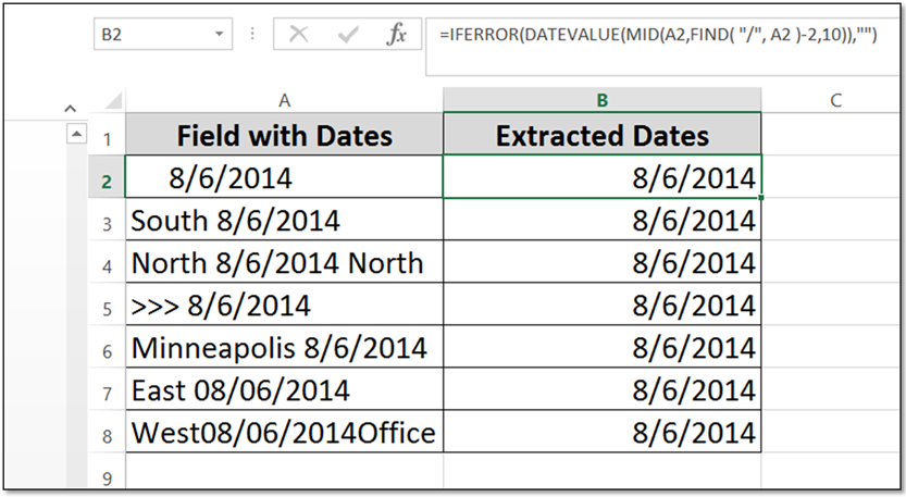
Let’s say that you wish to extract the dates from a less-than-ideal set of data.  For example, the Date Field may be mixed with text, spaces, symbols, or some combination.  So, what can you do with this unruly data?  Happily, Excel provides many possible solutions!

One way is to create a special formula that scours the field, and returns the date.  By using the MID, FIND, and DATEVALUE functions, most any irregular data can be handled with ease.  By adding in the IFERROR function, you can also keep your spreadsheet clear of any distracting error messages.

Putting this all together, creates the following formula:  =IFERROR(DATEVALUE(MID(B4,FIND( "/", B4 )-2,10)),"") which, as illustrated in the example below, neatly extracts the dates from the unconventional data contained in Column A:

There are, of course, typically numerous ways to achieve any result in Excel, and this is true in this case.  It is, however, one nifty little way to extract your dates from many types of unorthodox fields of data that you may have to work with in the future.  Try it some time when you need to Find Your Data!

A Review of Paste Special

Paste Special is one of those Excel tools that, due to its vital attributes, is good to occasionally review its many features.  It is unfortunate that more Excel users are not aware of the many advantages Paste Special brings to the everyday tasks in spreadsheets, so we are taking another look at it today.

There are no less than 17 Cool Things you can do with Paste Special.  To find it, simply copy something on your worksheet and Right-Click. Paste Special will be near the top of the dropdown list.

Here are the Top 5 Ways I use Paste Special on a regular basis:

1.  Paste Values: Simply copy the results of formulas, and Paste the Values in a new range of cells.  Great for getting rid of the formulas that created the data.

2.  Paste a Link: Merely copy a cell in another worksheet, click the Paste Link button on bottom-left of the Paste Special dialogue box and, Bamm, you can paste the dynamic link to a new location.

3.  Paste Validation: Easily copy a cell or range that has Validation applied, and paste that validation only to a new cell or range.  Incredibly useful at times!

4.  Multiply or Divide: You can copy a value and use Paste Special to multiply or divide an entire existing range of numbers.  Great for updating data or doing what-ifs!

5.  Transpose: You can easily transpose a column into a row, or a row into a column.  Quick and easy tool for those of us (like myself) who have a change of mind.

There are, of course, many other ways that Paste Special can come to your rescue.  If you are not a regular user of this marvelous tool, check it out some time and see what it can do for you!

Excel Navigation

It is a given that Efficient Navigation in Excel can save you time and even a little frustration.  Even discovering and using one or two new tricks can save you several hours over the course of a year.

Here are three ways to accelerate your ability to traverse the seas of your workbooks:

1.     Jump to the End or Start of a Column
If you work with very large worksheets that contain thousands of rows of data, you may occasionally find yourself far from the beginning of your column.  The comparative drudgery of scrolling back to the top can be easily overcome by using CTRL + ↑.  The opposite (CTRL + ↓) takes you immediately to the last nonblank cell in your column.

Note:  If you combine the SHIFT key with the foregoing, you will instantly select all contiguous date (Cool!).

2.     Jump between Worksheets
If you use this technique, you know that moving from one worksheet to another doesn't necessarily entail using your mouse.  You can move to the worksheet to the right by clicking CTRL + PGDN, and as you probably would guess, you can pop to the worksheet to the left by pressing CTRL + PGUP.

3.     Use the Name Box for Quick Navigation
Let’s say you have a very large worksheet, and you know that you want to go to the start of your list of California offices in Cell QM22879.  Rather than slogging down to the cell with your mouse, you can simply insert the cell address in the Name Box, click, and Bamm, you are there!

Take 5 minutes to master these three simple shortcuts, and see if they don’t save you a bit of time this month.  Who knows, you might be able to leave the office a few minutes early…

DAYS of Our Lives

How Excel handles dates and anything having to do with The Days of Our Lives, is always interesting to me, as it can at times be a bit less than intuitive.  For instance, simply subtracting two dates may give you the number of days between the dates, or it may create an error.  So what should you do?

The new DAYS function which was first introduced in Excel 2013 can help assure that you are getting the results you are seeking.  It is, of course, not terribly sophisticated, but it can come in handy at times.  One of the key features is that if either one of the date arguments is text, the DAYS function automatically kicks in the DATEVALUE function and returns an integer date.  

The syntax is:  =DAYS(end_date, start_date)

A simple example is shown below, where the formula, =DAYS(C3,B3) has been entered in cell D3 producing the result 196.

 

For something a little bit more interesting, let’s say you have a workbook that you use daily, and you would like to have a continually updated note of how many days it has been since the beginning of the current year.  Here is an example of an easy way to do this using the DAYS function, along with the TODAY function.  The formula, =DAYS(TODAY(), B2) is placed in cell C2, and automatically updates (pretty cool, eh?) every day:

The DAYS function.  Helping you avoid being in a DAZE in Excel (I know, I know, I have no shame…).