A Review of Paste Special

Paste Special is one of those Excel tools that, due to its vital attributes, is good to occasionally review its many features.  It is unfortunate that more Excel users are not aware of the many advantages Paste Special brings to the everyday tasks in spreadsheets, so we are taking another look at it today.

There are no less than 17 Cool Things you can do with Paste Special.  To find it, simply copy something on your worksheet and Right-Click. Paste Special will be near the top of the dropdown list.

Here are the Top 5 Ways I use Paste Special on a regular basis:

1.  Paste Values: Simply copy the results of formulas, and Paste the Values in a new range of cells.  Great for getting rid of the formulas that created the data.

2.  Paste a Link: Merely copy a cell in another worksheet, click the Paste Link button on bottom-left of the Paste Special dialogue box and, Bamm, you can paste the dynamic link to a new location.

3.  Paste Validation: Easily copy a cell or range that has Validation applied, and paste that validation only to a new cell or range.  Incredibly useful at times!

4.  Multiply or Divide: You can copy a value and use Paste Special to multiply or divide an entire existing range of numbers.  Great for updating data or doing what-ifs!

5.  Transpose: You can easily transpose a column into a row, or a row into a column.  Quick and easy tool for those of us (like myself) who have a change of mind.

There are, of course, many other ways that Paste Special can come to your rescue.  If you are not a regular user of this marvelous tool, check it out some time and see what it can do for you!

Excel Navigation

It is a given that Efficient Navigation in Excel can save you time and even a little frustration.  Even discovering and using one or two new tricks can save you several hours over the course of a year.

Here are three ways to accelerate your ability to traverse the seas of your workbooks:

1.     Jump to the End or Start of a Column
If you work with very large worksheets that contain thousands of rows of data, you may occasionally find yourself far from the beginning of your column.  The comparative drudgery of scrolling back to the top can be easily overcome by using CTRL + ↑.  The opposite (CTRL + ↓) takes you immediately to the last nonblank cell in your column.

Note:  If you combine the SHIFT key with the foregoing, you will instantly select all contiguous date (Cool!).

2.     Jump between Worksheets
If you use this technique, you know that moving from one worksheet to another doesn't necessarily entail using your mouse.  You can move to the worksheet to the right by clicking CTRL + PGDN, and as you probably would guess, you can pop to the worksheet to the left by pressing CTRL + PGUP.

3.     Use the Name Box for Quick Navigation
Let’s say you have a very large worksheet, and you know that you want to go to the start of your list of California offices in Cell QM22879.  Rather than slogging down to the cell with your mouse, you can simply insert the cell address in the Name Box, click, and Bamm, you are there!

Take 5 minutes to master these three simple shortcuts, and see if they don’t save you a bit of time this month.  Who knows, you might be able to leave the office a few minutes early…

DAYS of Our Lives

How Excel handles dates and anything having to do with The Days of Our Lives, is always interesting to me, as it can at times be a bit less than intuitive.  For instance, simply subtracting two dates may give you the number of days between the dates, or it may create an error.  So what should you do?

The new DAYS function which was first introduced in Excel 2013 can help assure that you are getting the results you are seeking.  It is, of course, not terribly sophisticated, but it can come in handy at times.  One of the key features is that if either one of the date arguments is text, the DAYS function automatically kicks in the DATEVALUE function and returns an integer date.  

The syntax is:  =DAYS(end_date, start_date)

A simple example is shown below, where the formula, =DAYS(C3,B3) has been entered in cell D3 producing the result 196.

 

For something a little bit more interesting, let’s say you have a workbook that you use daily, and you would like to have a continually updated note of how many days it has been since the beginning of the current year.  Here is an example of an easy way to do this using the DAYS function, along with the TODAY function.  The formula, =DAYS(TODAY(), B2) is placed in cell C2, and automatically updates (pretty cool, eh?) every day:

The DAYS function.  Helping you avoid being in a DAZE in Excel (I know, I know, I have no shame…).

Customizing Excel for You!

Excel is very smart.  Occasionally, however, it needs your help in understanding how you want it to work (after all, it can’t read minds or anticipate all needs for all users).

One of the ways that it needs your help is when you have Special List requirements.  As we all know, Excel has several familiar Built-in Lists, such as Sunday-Saturday, Jan-Dec, etc.  Your own user-defined lists can be very practical, however, as they can be used for sorting or Auto-Filling your data.

 

Using Excel 2013 for Illustration, Here is What You Do:

1. Go to File/Options and then click the Advanced option
2. Scroll down to the General category, and click the Edit Custom Lists button
3. In the Custom Lists box, click NEW LIST, and then type the entries in the List entries slot
4. When the list is complete, click Add
5. Click OK

An Easier way, (especially if you are dealing with a larger list), when using the Custom Lists dialogue box, Import it directly from a completed column list:

 

The Bonus in all of this is, of course, is that your Custom Lists are added to your computer's registry, so it is always available for use in other Excel workbooks.

Give it a try sometime.  You may find that Custom Lists will give you a New Ride in Excel!

Happy July 4th!

Happy July 4^th, Everyone! I hope you are enjoying the holiday (with sincere apologies to my friends in the UK…)!

I am a great believer in Having Fun!  You’ve got to have fun in your life because, regardless of how you look at it, it’s all a game!  Since this is a holiday week here in the U.S., I thought it would be fun to revisit the somewhat impractical Excel function, ROMAN.  This function, rather obviously, converts ordinary Arabic numbers into Roman Numerals.  Useless, you say?  Well, still fun to play around with.

The syntax is as follows: ROMAN(number, type) or simply ROMAN(number) if you wish to accept the Classic Roman numeral format.

Let’s say you have the number 2014 in cell A1, in cell B1, insert the formula ROMAN(A1), and your result is MMXIV.  For a little more fun, try it out with a formula that calculates your current age:  =DATEDIF(birthdate, TODAY(), “y”).

Putting your birthdate in A1, and the How Old am I in Roman Numerals formula in B1 it would be expressed as =ROMAN(DATEDIF(A1,TODAY(),"y"))

If you were born on September 3, 1974, the result shown would be your age of 39 expressed as the Roman numeral, XXXIX.  What fun!

 

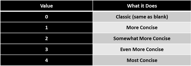
If you want to explore this function a bit more, you can use the Second Argument option with the ROMAN function, which converts your results to varying levels of brevity.  Note the following values in the table below:

 ROMAN Numerals.  A little Fun for your Fourth of July (that is, if you are a geek like me…).  Cheers!

Text to Columns

Today’s topic concerns a tool that is very basic to use, but one which a great many of Excel users never use.  From several conversations I have had with other Excel people over the years, it appears that few are aware of the Text to Columns feature in our favorite program.

As we well know, data isn’t always presented in the most ideal formats.  There are frequently times when it comes from a variety of sources outside of Excel; Sometimes even from Word documents, Gasp!  So how does the Text to Columns tool work?  Here is what you do:

For sake of illustration, let’s use the following string of numbers (remember, this is intentionally rudimentary…) that you may find in a Word document or any other numerous sources:

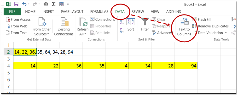
14, 22, 36, 35, 64, 34, 28, 94

 
1.     Simply select the string, copy it, and paste it into a cell in Excel (in this example, A2 was used)

2.     Select the cell and click on the Text to Columns icon on the DATA ribbon

3.     The Convert Text to Columns Wizard will appear giving you the following two major options:

a.     Delimited – Characters such as commas separate each field

b.     Fixed width – Fields are aligned in columns with spaces between each field

4.     In our example, we choose Delimited since our numbers are separated by commas

5.     Following the next steps in the Wizard gives you the choice to pick your desired format:

a.     General

b.     Text

c.      Date

Badda-bing!  It really is that simple to get your data into Excel in proper alignment and format.  The Text to Columns tool may be just the ticket for that task just around the corner!

Gantt Charts in Excel

When used correctly and consistently, Gantt Charts can be invaluable tools to managers, analysts, and employees in the front lines.  So what, exactly, are Gantt Charts?

Well, first of all, they are a comparatively simple bar charts that illustrate and track the evolution of a project.  Developed by a management consultant by the name of Henry Gantt back in the early 20^th century.  These respected charts clarify the start and finish dates of a project’s elements, and can be easily grasped a quick glance.  Groundbreaking at the time they were developed, Gantt charts are considered mainstream today.

Along with Microsoft Project, there are several specialty software solutions for producing these charts.  For many, however, good old Excel handles this quite satisfactorily, thank you.  Here is what you should do:

1.     Open a New workbook in Excel (version 2013 is recommended)

2.     Type in “Gantt” in the Search for online templates box

3.     Choose the Project Planner template and click Create

The Project Planner Gantt chart template will then open, and you can customize it to suit your business and aesthetic needs.  Please Note: You can access Manage Rules under Conditional Formatting on the Home ribbon and revise the formatting and range of the chart.  I recommend that you modify the formatting, as the default, IMHO, is rather ugly.

With these easily created and used Excel Gantt Charts, you can quickly see where each activity is according to plan.  Give it a try the next time a Big Project comes by!