MicroGraphs for All!

As many of you may know, “Sparklines” first appeared in Excel 2010.  Sparklines make it quick and easy to create readily-intelligible micrographs within the cells of your Excel spreadsheets that highlight important details of your data.  They have the same utility as traditional graphs and charts, but they have the additional benefit of being incorporated right next to the data which you wish to illustrate.

Well, that’s pretty cool, but what if your company is still using Excel 2007 or even Excel 2003, (a recent survey showed a significant number of companies still using these older versions), and you want to use some Cool Little Micrographs on your spreadsheets?  What can you do?

A very effective way to make these engaging little graphs is to incorporate an unpretentious formula and a touch of conditional formatting.  Let’s look at how this can be done…

Let’s say you have the Producers of your company’s products in Column A as illustrated below, and in Column B you have the Units Sold each producer has sold. Here is the simple formula you should put in Cell C2 (and then copy it to C8):

= REPT( “l” , B2/1,000) 

For each Approximate Count of One Thousand, the formula puts an old-fashioned Hash Mark, (using a bold, simple font works well), in Column C. With a bit of Conditional Formatting, the result is a clean, professional report that integrates a MicroGraph! Using these elementary graphs makes your data Visually Comprehensible and enhances the user’s understanding of what is being said in your Excel reports.

If you are using a pre-2010 version of Excel (or even if you are using a more contemporary version), try it out sometime and see what you think. It’s good stuff!

Happy Thanksgiving All!

Sales Analysis with Coefficient of Determination

The correlation of data can be an extremely worthwhile endeavor for any business analyst. Adding some graphical depiction of your analysis can make it even better.

One of my favorite charts and accompanying functions are Scatterplot (XY) Chart and the Coefficient of Determination function. This quick analysis combo truly should be in your Excel Tool Belt!

Let’s say, for instance, that you want to do some speedy research into the efficacy of your sales advertising. Perhaps you want to know whether it is typically better to spend advertising dollars on Tuesday or Thursday.

First determine your ad effectiveness on Tuesdays by selecting data from those days and making a Scatterplot Chart.  Then do the following:

1. Right-click on one of the data points and
2. Choose Add Trendline
3. Right-click the Trendline and choose Format Trendline
4. Format the Trendline to your preferences and
5. Put a Checkmark next to Display R-squared Value on Chart

 

The R-squared value is your Coefficient of Determination (COD) that will tell you how strong your data on your two axes. In the example above, the COD value is .74 (or 74%) representing a strong correlation between spending advertising dollars on Tuesdays and increased sales.

Then simply do the same for your Thursday data, and compare the size of the CODs. If you get, for example, a Coefficient of Determination of 74% on Tuesday and 41% on Thursday, Hey, it’s a no-brainer!  Spend your money on Tuesdays!

Try using a Scatterplot and Coefficient of Determination sometime when seeking the strength of a correlation of data sets or multiple sets. It is Fast and Effective. Just don’t tell anyone how Easy it was!

Truly Blank?

Today’s topic may initially seem a bit obscure, but let me assure you, if you are ever faced with some odd results from what appears to be routine data, it is something to consider.  Let’s say that you have what appears to be a number of blank cells in the range on which you are performing a calculation.  If you are getting strange results, you might ask yourself, “Are the blank cells actually blank?”  The truth is that it is Not Always Easy to know whether a cell or cells in Excel are Truly Blank!

The reason it is difficult to immediately know if blank cells are truly blank is due to the fact there are several ways of Hiding Data through:

o   The use of identically-colored fonts

o   Empty-string results of a formula

o   Masking the data with the use of Custom Formatting (three semicolons: ;;; )

It can cause Mayhem with your calculations.

To detect this Invisible Data, there are at least a couple of techniques.  Assuming your cell in question is A1, you can:

1.      Simply insert this Function in an adjacent cell:  =ISBLANK(A1) 

o   If the cell is Blank, it will return True; if it is Not Blank, it will return False

o   Copy the simple formula to include the rest of the range you are investigating

2.      A second technique it the use an IF Statement as follows:  =IF(A1<>"","Not Blank", "Blank")

o   This IF Statement obviously returns Blank or Not Blank

 

o   You can then take the appropriate action with the Not Blank cells

By determining if your cells are Truly Blank, you can help Avoid Quirky Results on your worksheet.  And, as Martha Stewart might say, “That’s a good thing…”

Keeping Things Safe

How many times have you heard or read that you should routinely back up your data on your computers?  Well, protecting your Excel work can be similarly important. 

Perhaps you are asking “Why is this important?” Maybe you have never done this, and never had a problem. That may be just fine if you are the only one using one of your Excel masterpieces, but if are sharing your work (and most of us probably are) with others there will come a time when the others will want to “Experiment” with your formulas and format. Don’t let this happen!  The construction of your workbook may have taken dozens of hours to create, and there is the potential for substantial ruin!

Happily, Excel has built-in Protection Tools to help us all out.

Let’s take a look at Excel 2013 for a How-To Example (other versions are similar):

Protecting and Unprotecting a Worksheet with a Password

1. If there are specific cells that you wish to enable users to modify (such as a Data Entry Range in a dynamic report), go to the Review tab and select the Allow Users to Edit Ranges in the Changes group and select the range you wish to keep accessible. In the example below, cells B5:B14…

2. Next, click the Protect Sheet button in the same dialogue box. Excel in turn opens a Protect Sheet dialog box (see below), where you can Assign a Password, and select the Permissions you wish to be available to the users.

3. Click OK

You can easily Unprotect the worksheet with the password anytime you wish to make changes. And, of course, as this can cause a business disaster (people have been fired for losing this), Be Sure to Keep Track of the Password. This should barely warrant mentioning, but it does happen.

One Last Important Note: Protecting your worksheets is Not making it absolutely Secure.  It is not ample protection to prevent users from accessing confidential or sensitive data, and any backyard hacker can break it.  It is for casual protection.

Protecting Your Worksheets.  Certainly a Best Practice for any Excel practitioner, and one worth your time. Give it a try, and find out how easy it is to add a bit of protection to your hard work.

The Advanced Filter

As you may well agree, there are a great many powerful gadgets in Excel that are seldom used.  The Advanced Filter is just one such example of an often-overlooked, but enormously useful tool.

The beauty of this tool is that it is, well, Advanced.  You can, however, use it in comparatively simple ways to get an immediate understanding of how it works.  We will take a look at a couple of examples of how to use the Advanced Filter.

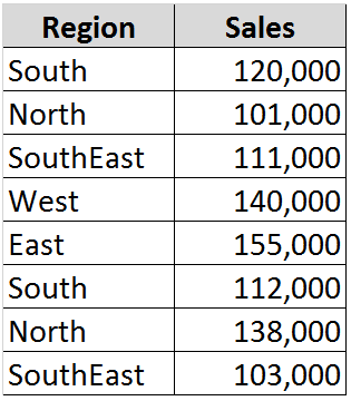
First of all, we will assume you have the following small database (keeping in mind, of course, that this tool works equally well with databases containing thousands of records):

 As is the case with any well-designed database, each field (column) has a header/name.  Not surprisingly, this is a necessity when using this tool.

Next, we will access the Advanced Filter by going to the Sort & Filter group on the Data tab, and clicking on Advanced. 

In the List range field put the location of your database (in this case it is B3: C11).

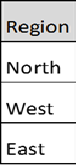
For the Criteria range, let’s assume you want to see all of the sales for the North, West, and East regions, and you want to place this filtered result below your database (use B13 for a starting point).  Simply set up a range such as in the following cells E3:E6 (or wherever you wish):

Your result will appear as follows in your chosen location:

Okay, Cool, but don’t stop there; you can use multiple field names and criteria to extract a wealth of information in a mere three clicks.

When you’re ready to Graduate up to another level, give the Advanced Filter a try.  I think you will like it!

Automatic Fun!

It is probably fair to say that the vast majority of us appreciate Spellcheck in the apps we use on a daily basis (except, of course, when it chooses to do weird substitutions…).  What many Excel pros are missing, however, is that they can Customize automatic corrections with the highly useful, (but typically underutilized), Autocorrect tool.

This is particularly useful if you find yourself typing long (or even moderate) Boilerplate phrases that are tedious and time-consuming.  For a brief example, let’s say you work for Harley-Davidson Motor Company and the company policy is that no abbreviations of the corporate name be used in correspondence.  Typing the entire name every time you do any kind of spreadsheet or correspondence may not seem terribly onerous, but it can be a small irritation (and who needs that!).

The way you set up a phrase (company name in this case) in Autocorrect may seem like a bit of a chore, AutoCorrect can make this is as easy as typing HDMC.

Here is How You can Set this Up:

1. Go to FILE and select Options from the bottom of the column

2. Choose Proofing and click on the AutoCorrect Options button

4. In the Replace box, type HDMC

5. In the With box, type Harley-Davidson Motor Company

6. Click Add and then OK. That’s all there is to it!

But wait! There is a chance for some Tricks along with the Treats.  Many of you know the gag of accessing a fellow employee’s computer, and switching the mouse controls from (for example) to left-handed from right-handed, and then watching the bewilderment of the user.  Well, you can also have some fun (all very adolescent) with a person with Autocorrect. 

Let’s say you have a friend named Jim at work (or whomever). While he is away from his computer, go into AutoCorrect and enter Jim in the Replace box and Easy Rider in the With box. This can be done in Word too, of course, and he will perhaps think he is channeling the Harley experience.  (Just be sure you have him do this in your presence, so he doesn’t unnecessarily embarrass himself.)

Autocorrect.  Useful for productivity and a bit of mischief. 

Never Retire!

Since I have my 65^th birthday coming up in a few days, I thought it would be interesting to take a look at a really cool formula or two that calculates when you are going to retire.  This can be a useful tool if, for example, you work in Human Resources or if you are doing Financial Planning.  It can also be entertaining if you just like to Daydream about days in the future when all you are concerned about is laying on the beach (getting even more wrinkly…).

I, for one, have absolutely no desire to retire anytime soon, since I enjoy teaching, blogging, and instructional design too much to give it up (besides, I look like I’m only in my 40s, Ha!).

If you have worked with Excel for some time, you know that it can be a bit quirky when it comes to handling dates.  Today, however, we will look at a couple of truly elegant ways of calculating your retirement date based on the Retirement Age you choose and on your Date of Birth.

In our first example, we’ll assume that the person’s birth date is in cell A2 and retirement age is 66.  In cell A3 create a formula as follows:

=DATE(YEAR(A2)+66,MONTH(A2),DAY(A2))

Another, even shorter, formula that you can use is the following (please note that you will need to format your cell as a date after using these formulas):

=EDATE(A2,66*12)

 

Well, there you have it; two uber-cool ways for Calculating Your Retirement Date. Now pardon me while I get back to work (laying on the beach can wait…).