INDEX/MATCH vs. VLOOKUP

I have a group called Excel Enthusiasts (catchy title, eh?) on LinkedIn that I started several years ago.  It currently has over 16,000 members from over 60 countries.  Recently, one of the leading discussions has been on which is better, VLOOKUP or INDEX/MATCH. 

Clearly, VLOOKUP is by far the most frequently used function in this instance, primarily because it is the more unassuming formula, but also because most Excel users simply don’t understand how to use the INDEX/MATCH combination.

The major drawback of VLOOKUP is it requires a static reference in the form of the first column.  Not very cool.  INDEX/MATCH on the other hand, is much more flexible, allowing you use whichever column you choose for your reference.  Much cooler.

Let’s take a look at a simple example using the Illustration below:

Let’s say you wish to create a Code Retriever.  MATCH returns the Row Number of the location in an array of value you specify. Using the example above, the number “4” is returned by the formula:

=MATCH("Tampa", $A$2:$A$8,0)

INDEX, on the other hand, returns the Value that you identify by row number in an array. Using the example above, “Tampa” is retuned by the formula:

=INDEX($A$2:$A$6,4)

Combining the INDEX and MATCH functions is where the Real Power comes in. Let’s say we want the Code for San Diego. We can set up a Code Retriever as shown in cells E1:F2, by inserting the following formula in cell F2 (This will return "141"):

=INDEX($C$2:$C$8, MATCH(E2, $A$2:$A$8, 0))

Using the MATCH and INDEX functions together is truly a Powerful way of extracting data when you need it. Once you try it, you may never go back to VLOOKUP again!

Validation is Good Stuff...

I am currently teaching an Excel class to a fine group of intermediate-advanced users.  One of the topics we are reviewing is the many uses of Validation. 

Validation can be useful in many arenas, including the maintenance of Integrity of your data, (we’ve all heard of GIGO – Garbage In Garbage Out), convenient Drop Down Boxes, informative Popup Alerts, and much more.

Maintaining Integrity

If you know that only certain data should be entered in a range, you can easily control this by using one of the many controls in the Allow dialogue drop down.  You can control size or range of numbers, text considerations or, as in the example below, which words can be entered (in this case, True or False…).

Drop Down Boxes
Drop down boxes can add interactivity and professionalism to your worksheets.  By choosing List in the Allow box, you can select a range of cities, employees, customers, companies, whatever you find useful.  In the example below, as list of sales representatives was selected.

Popup Alerts

By using boxes included on the Input Message tab, you can create a Popup Message whenever a user clicks on a cell within the range this Validation is used.  This can be further useful in assuring that the proper information is being put into your database, and it helps jog the memory of the user entering the data.

Validation.  Many uses, many benefits.  Really Good Stuff!

Frequency Functions and Tables

Array Functions are one of those categories of Excel tools that most Excel users have never heard of, and mystifies most of those who have.

These mysterious functions can be quite useful, however, and when you learn how they are activated, you will laugh at how easy (albeit unusual) they are to use.

If you want to do some analysis on how frequently values within particular ranges occur (rather than looking at each individual occurrence), for instance, an excellent solution in Excel is the Frequency Function.  This valuable tool works as an Array Function that counts the number of values that occur in each specified interval (or “Bins”, as they are typically called).

The FREQUENCY Function syntax is as follows:
        FREQUENCY(DataArray, BinsArray)

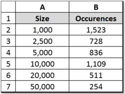
The function utilizes a database for a source, and is entered as an Array formula after you select a range of adjacent cells (B2:B7 in our example) into which you want the distribution to appear. After you select the data and bins arrays, press CONTROL+SHIFT+ENTER (this is what mystifies many users…).

The following example shows the “Bins” under the heading Size and the Frequency of claims within each range under Occurrences:

Special Note: The number of elements in the returned array is one more than the number of elements in bins array. The extra element in the returned array returns the count of any values above the highest interval.

Illustrations of key applications of the Frequency Function will be explored in future blogs that will be published soon.  In the meantime, take a 5-minute look at this vital tool.  You may find that it is not all at mysterious…

AutoFilter Tricks

This is a great little technique to start your year of Excel use off right.  The AutoFilter tool is a sometimes underused and under-loved convenience that has some built-in tricks that many Excel users are simply unaware of. 

Let’s look a Totally Cool example:  First select any cell within your table or database, go to Data, choose the Filter menu, and click on AutoFilter. AutoFilter Arrows will appear at the top of each column, allowing you to filter on whichever column you choose.

Okay, good.  Most of us know all about that, but what kind of Cool Tricks can you do after that? 

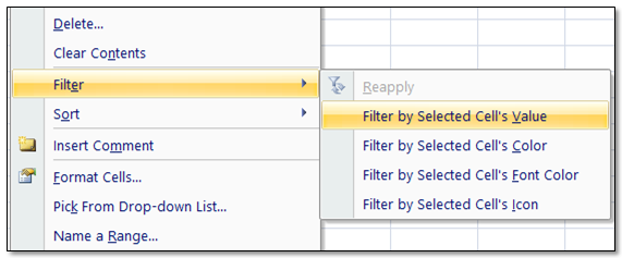
Well, let’s say you want to filter/sort a table which includes the sales figures for several reps and regions.  If one of your regions is called SouthEast and you want to see just the sales from that part of the country, for instance, you can simply right-click on any cell which has “SouthEast” in it, and choose Filter by Selected Cell’s Value from the secondary Filter menu.

 

Bamm!  Your data is instantly filtered to show only that region!

Not cool enough for you?  As you can see by the screenshot above, you can also use this technique to filter by the cell’s Color, Font Color, or Icon!  All in the blink of any eye! 

You can also create a great variety of Custom AutoFilters to manipulate your data, but for On-the-Fly Wizardry try one of these handy right-click approaches and see how many of your Excel user comrades raise their eyebrows.  As I always say in my classes, “Right-Click (with Filtering or most other things in Excel) is Our Friend!”

 

Happy New Year, All!

Links are Cool!

I think we all agree that Charts are Engaging, Readily Informative, and Cool. But is there a way to make them Even Cooler, you ask?  Oh, yeah, Man!

For instance, let’s say you have a chart of sales figures that is interactive relative to which sales representative you choose from a Dropdown Box.  An easy way to do this is by using Validation. Simply select the cell in which you want the dropdown, choose Validation / Allow List and then select a range for your Source of dropdown entries.  Presto! Instant DropDown Box!  By combining a dropdown and elements such as a VLookup function, you can create a powerful and interesting report in Excel

But, would it be possible to have the Title of the Chart Change to reflect the value chosen? Yes, indeed! (It is so easy, you’ll laugh…)

Here is How You Do This:

1.    Select the Chart Title

2.    Go to the Formula Bar and type an Equals Sign: “ = ”

3.    Then Select the Drop-Down Box Cell to which you want to link

4.    Note: The final cell reference formula should look something like: “=Sheet1!$B$3”

How Totally Cool is that?!?!  Now every time you change the Name or Value in the Drop-Down, the Chart not only updates its graphical display of data, it Automatically Updates its Title! 

With this trick you can WOW your boss, your colleagues, your employees, even your dog or cat!  Give it a try!

Happy New Year, All!

Graphics in Excel

Excel users can be a funny lot.  Many of us tend to think of anything outside of cold, hard data is a waste of time and, moreover, rather frivolous.  Data and, more importantly, Information is, of course, what Excel is all about.  The thing is, though, it doesn’t have to be dull.

Excel is actually loaded with an array of graphics tools that can make your spreadsheets more engaging and readily informative.  Let’s look at some ways this can be done:

 Interesting Charts

Using some lively graphics can add real Pop to an otherwise sufficient chart.  Plotting Surfing Days in Southern California?  Use Surfboards in your chart!

 

SmartArt

You can find SmartArt in the Illustrations group on the Insert ribbon.  SmartArt quickly enables you to create diagrams of Org Charts, Processes, Cycles, and much more.

 

WordArt

Enter some eye-catching stylized text with Word Art objects.  Just click on the WordArt dropdown button from the Text group and choose a style that appeals to you.  You can resize and drag this text to any part of your worksheet.

 

Shapes

Let’s not forget the readymade shapes that add Functionality, as well as engaging panache to your Excel workbooks.  You can add Words and Hyperlinks to these easily-created shapes, enabling the user to navigate to anywhere you wish them to go

There are several other ways to add graphics to your Excel masterpieces, of course, and they can indeed add a touch of brilliance to your work.  I encourage you to try them out on your next report.  I’m sure your users will approve!

Happy Holidays All!

Medical Records and Excel

Having been diagnosed with a bit of pneumonia a couple of days ago, and getting a laundry list of medications to manage, it occurred to me that Excel would likely be a good friend in this regard.  So I created a simple spreadsheet/checklist to help me keep track of the what and when of my meds.

But wait!  Excel can do so much more: A brief amount of investigation revealed that, indeed, Excel offers a great deal of potential premade assistance to individuals wanting to track their medical concerns. Included in this group are the following templates:

·       Weight Loss Tracker with BMI

·       Blood Pressure Tracker

·       Calorie Amortization Schedule

·       Blood Sugar Tracker

·       Exercise Planner

·       Fitness Progress Tracker

There are many third-party predesigned dashboards, databases, and templates created for medical professionals as well.  A few of the most notable are those from:

·       Chandoo

·       Softonic

·       Tableau Software

In addition to a these out-of-the-box suggested formats, good old Pivot tables can be a tremendous boon, especially for medical professionals.

There are applications in Excel that can touch a myriad of facets of our personal, as well as our professional lives.  This is simply one more way that Excel can be of assistance.