AutoFilter Tricks

This is a great little technique to start your year of Excel use off right.  The AutoFilter tool is a sometimes underused and under-loved convenience that has some built-in tricks that many Excel users are simply unaware of. 

Let’s look a Totally Cool example:  First select any cell within your table or database, go to Data, choose the Filter menu, and click on AutoFilter. AutoFilter Arrows will appear at the top of each column, allowing you to filter on whichever column you choose.

Okay, good.  Most of us know all about that, but what kind of Cool Tricks can you do after that? 

Well, let’s say you want to filter/sort a table which includes the sales figures for several reps and regions.  If one of your regions is called SouthEast and you want to see just the sales from that part of the country, for instance, you can simply right-click on any cell which has “SouthEast” in it, and choose Filter by Selected Cell’s Value from the secondary Filter menu.

 

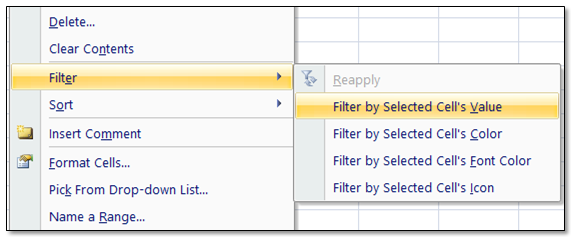
Bamm!  Your data is instantly filtered to show only that region!

Not cool enough for you?  As you can see by the screenshot above, you can also use this technique to filter by the cell’s Color, Font Color, or Icon!  All in the blink of any eye! 

You can also create a great variety of Custom AutoFilters to manipulate your data, but for On-the-Fly Wizardry try one of these handy right-click approaches and see how many of your Excel user comrades raise their eyebrows.  As I always say in my classes, “Right-Click (with Filtering or most other things in Excel) is Our Friend!”

 

Happy New Year, All!