Picture Charts!

There is no doubt that Excel provides a considerable array of Chart Types to choose from. There are times, however, when you may want to Add a Bit of Pizazz to your charts. One of the coolest ways to do this is by Replacing the Series Element (Columns or Bars work the best) with a Graphic.

You can easily Add Impact to your charts by doing the following:

1. Copy a Graphic (simple images work the best) to your clipboard
2. Create your Chart using columns or bars
3. Select the Chart Column or Bar Series
4. Go to your Home Tab and Paste the image
5. Bonus: Format the Data Series by going to Series Options and choosing 0% Gap Width

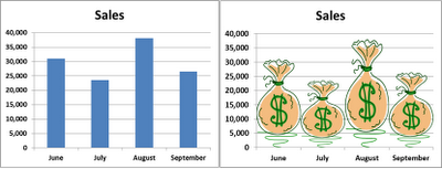
Since I live in southern California, I chose a Surfboard Graphic for my Surfing Days Chart above. To demonstrate the difference this can make, I did a Side-by-Side illustration below. I chose a Bag of Money to replace the Boring column to depict the sales by month.

Picture Charts. Another way to Add Interest and Impact to your Excel worksheets.

Surf’s Up!

Excel on the Cloud

As any technophile knows, The Cloud is the Major Buzz these days. It seems that everyone is scrambling to say, "Me Too" in their quest to capture your traffic and business via cloud-based apps or, as with Microsoft's Office 2013, span both traditional approaches and the cutting edge.

My current favorite Cloud Solution is indeed supplied by the venerable Microsoft. By placing your Excel workbooks on SkyDrive, they can be shared (at your discretion) with the world. All you need to do is go to your SkyDrive, right-click the document, and then click Share. Type the email address of the person you want to share the workbook with, and Bamm! Done!

But Wait! What makes it Really Cool in this instance is that the other parties with whom you are sharing Do Not even have to have Excel on their computer! That Totally Rocks!

Other favorites include the iPad Numbers app. Workbooks created or edited in Numbers can be converted to the Excel format, and shared on iTunes, DropBox, and other cloud-based facilities.

Google Docs is also hugely adaptive and beneficial for anyone (or any organization) who is on a budget, and still wants reasonably high functionality and ease of collaboration.

So, what about me, am I personally Truly embracing the mobile world and the cloud? Well, as an evidenced by this week's blog which I have written entirely on an iPad while awaiting an appointment, yeah, I guess you could say that I am!

Happy Thanksgiving, All!

What’s the Dif, Man?

Back in July of 2010, we looked at the obscure, and curiously undocumented function, DATEDIF. Microsoft, in all of its wisdom, (small amount of gentle sarcasm here), has chosen not to include documented information on this Essential Function in Excel. Over the past 5 years of this blog, this topic has been one of the readers’ favorite.

As any longtime user knows, the way Excel handles dates can be a bit puzzling at times. Finding the Difference between two Dates, for instance, is not readily intuitive. Here is where DATEDIF shines!

The Syntax of the Function is as Follows:

=DateDif(First Date, Second Date, Time Interval)

Where the Time Interval is expressed as follows:

d (Days) = Number of days between the dates
m (Months) = Complete calendar months between the dates
y (Years) = Complete calendar years between the dates

Important Note #1 (you don’t need this craziness): The Second Date must be greater than the First Date, or you will get a Number Error.

A novel application of this function is to nest the NOW() function into it and calculate a Person’s Age. The NOW() function returns the Current Date and Time, and when used with DATEDIF, it can produce an Excel calculator that many find amusing. (Note: the “BirthDate” can refer to an easily changed Cell Value):

=DateDif(BirthDate, NOW(), “y”)

Important Note #2: If you put the Time Interval in the function directly, be sure to put “quotation marks” around it (e.g. “m”). If you put it into the formula via a cell reference, do not use the quotation marks (e.g. the cell should contain m, not “m”).

You may well find a great many ways to use the DATEDIF function, which may lead you to wonder, Why is this Terrific Tool not documented? Ah, well, who am I to question the great Microsoft…

Go To Special

I have a question for you: Do you ever use Go To Special?

If you answered, “No” to the previous question, you are undoubtedly in the vast majority of other Excel users. You may find this to be a useful tool, however.

I’m quite sure that some time in your Excel career, you have found yourself wondering how you can locate certain types of cells within your worksheets. For example, you may have wanted to find the cells in your worksheet which contain Formulas, or perhaps those which have Conditional Formats.

You may be pleased to know that Excel provides a terrific Tool to help you locate these and many other Special Types of cells. The Go To Special dialog box can provide you with options you may not have realized that you have in Excel.

You can find this nifty tool on the far right of your Home Ribbon. Simply click on Find and Select and choose Go To Special. Once there you can choose Comments, Constants, Formulas, Blanks, Current Region, as well as many other choices.

Now that your cells have been selected, you can perform whatever operation you may see fit. This simple tool can save you a lot of time searching through your worksheets, and can inevitably Help You Prevent Errors.

Go To Special; A useful tool to have in your Excel arsenal!