Match and Index Revisited

Back in 2010, we took a look at the Power of using a table or database combined with the MATCH and INDEX tools in Excel. Due to the lack of use of these Fabulous Functions, (VLOOKUP is more popular, but less robust), today we will Reexamine how and why you should keep this technique in mind.

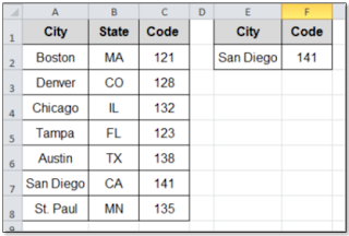
If you want something more versatile than VLOOKUP, MATCH and INDEX can serve as your humble servants. Let’s take a look at a simple example using the Illustration above.

For instance, MATCH returns the Row Number of the location in an array of value you specify. Using the example above, the number “4” is returned by the formula:

=MATCH("Tampa", $A$2:$A$8,0)

INDEX, on the other hand, returns the Value that you identify by row number in an array. Using the example above, “Tampa” is retuned by the formula:

=INDEX($A$2:$A$6,4)

Combining the INDEX and MATCH functions is where the Real Power comes in. Let’s say we want the Code for San Diego. We can set up a Code Retriever as shown in cells E1:F2, by inserting the following formula in cell F2 (This will return "141"):

=INDEX($C$2:$C$8, MATCH(E2, $A$2:$A$8, 0))

Using the MATCH and INDEX functions together is truly a Powerful way of extracting data when you need it. Once you try it, you will be Amazed!