Retirement Age

No, I’m not thinking of retiring anytime soon, but it can be useful to have a nifty little formula or two that calculates Retirement Age in Excel. This can be very useful, for instance, if you work in Human Resources, if you are doing Financial Planning, or if you just like to Daydream about days in the future when all you are concerned about is your golf score.

As anyone who has worked with the application for a long time will tell you, the way Excel handles dates is sometimes a bit less than intuitive. There are, however, a couple of elegant ways to calculate Retirement Age based on a person’s Date of Birth.

First of all, let’s assume that the person’s birth date is in cell B2 and retirement age is 65. One way to do our calculation as follows:

=DATE(YEAR(B2)+65,MONTH(B2),DAY(B2))

Another, even shorter, formula that you can use is the following (please note that you will need to format your cell as a date after using this one:

=EDATE(B2,65*12)

Well, there you have it; two slick ways for Calculating Retirement Age. Now pardon me while I daydream about golfing on Pebble Beach…

Combo Charts!

A good Rule of Thumb when making charts is, “If you have to think about what the chart is saying, it isn’t a good chart”. Combo Charts are a very effective way to improve your communication in your Excel Charts.

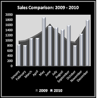
Although adding a Second Axis is a classic technique that is often applied with Combo Charts, it is not always necessary. For instance, let’s say you want to compare the sales figures for two years, and you want to be able to instantly see which months were more successful and which were less successful. This is quite easily done, and can be enhanced with a bit of thoughtful formatting.

Let’s Look at the Following Example:

1. Create a standard Column Chart using the table below:

2. This will produce the Difficult-to-Decipher (and rather ugly) Standard Column Chart as illustrated below:

3. Right-click once on any single column for the year 2009. This will select all of the columns for that year.
4. You can then select Change Series Chart Type and choose an Area Chart
5. Double-click on your chart, and bring up the Design Tab Tools.
6. Then take a couple of minutes to add some visual appeal by formatting your chart to create an easy-on-the-eyes chart similar to the one below:

That is all there is to it! You can easily create a Combo Chart that will greatly enhance your ability to understand your data and Communicate Effectively with your spreadsheet viewers. Very Cool!

Reference Please...

There are times when it is good to be able to automatically reference the Name of your Excel workbook or worksheet that you are doing your report on. If you wish to have the results in a cell refer to the Entire Name and Location of your worksheet and workbook, that is easy: You merely put CELL(“filename”) in any cell, and you get the entire kit and caboodle such as the following (yours may even be longer):

C:\My Documents\ExcelBlog2011\[Sales Report.xlsx]Sales 2011

But what if you want to just to have your cell reference the Name of the Worksheet you are on? This can be very useful when printing reports, and can be accomplished using the following formula:

=MID(CELL("filename", A1),FIND("]",CELL("filename",A1),1)+1,254)

Very nice, you say, but how does it work? Here it is broken down starting with the FIND function in the middle of the equation:

1. In this instance, FIND looks for the Right Square Bracket in the resulting CELL(“filename”, A1) string (please note that the cell reference “A1” is entirely arbitrary, and any cell reference will do).
2. MID looks in the same resulting CELL(“filename”, A1) string and uses the Start Number that was found in Step #1 above and Adds 1 (so you do not get the Bracket in your result).
3. The final argument, 254, merely allows up to 254 characters to be returned.

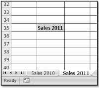
The final result is the Name of the Worksheet you are on, or in this case, Sales 2011.

Powerful Stuff! Copy the formula and paste it into your own worksheet to see how Cool this works.

Cheers!

Form Controls Rock!

There are few tricks in Excel that can make you into a Rock Star faster and easier than Form Controls.

Some of the main reasons Form Controls are useful include:

1. They are Intuitive for non-techies to use
2. They can be used to force users to choose one of your provided options and maintain database Input Integrity
3. They enhance your worksheet with a professional visual appeal, giving true Pizzazz!

Form Controls are quite easy to use and require no programming knowledge. They can be used to easily place values in worksheet cells, and make you Look like a Genius in the process.

These marvelous controls can be accessed in Excel 2007 or 2010 by:

1. Making sure that the Developer tab is on your ribbon tabs
2. Go to the Controls section and click on the down-arrow beneath the toolbox
3. Choose the Form Control you wish to use in your worksheet

You have your choice of Combo Boxes, Spin Buttons, Check Boxes, List Boxes, and much more.

For example, let’s say that you wish have a Check Box (or multiple check boxes) on your worksheet that will make a cell value either True or False. These responses can then be used in formulas that activate or manipulate other sections of your worksheet or workbook.

Check Boxes can easily be chosen and drawn on your worksheet with a click of the mouse. It is then a simple matter of Right-Clicking on the Check Box and choosing Format Control (this works similarly the other form controls as well.) You can then choose the cell or cells you wish to Link Your Control to and Format the Visual Style of your control

How Absolutely Rocking Cool is that! Take 5 minutes and make your Excel worksheets look like you spent hours of programming time on them. Give it a try – Add some Form Controls to your worksheet and give it some Bling!

More AutoFilter Tricks

When Excel 2007 debuted, it brought with it Enhanced Functionality to the AutoFilter tool. If you have a database or table with headings in the top row, you can use AutoFilter to do some very amazing, On-the-Fly feats!

First of all, let’s turn our data into a Table by selecting any single cell within the database, and clicking Ctrl+T. Bamm, we have a formatted table with AutoFilter turned on!

In older versions of Excel, your Autofilter choices were pretty limited, but with Excel 2007 and Excel 2010, you have a much greater variety of options available. For instance:

• With Text Fields, you can use the built-in Text Filters to display cells that Start with, End with, or Contain the text of your choice.

• With Date Fields, you can easily use the Date Filters to sort for records from Last Month, This Month, Next Quarter, or nearly any parameter you can imagine. If you do not see it as a premade option, you can simply create a Custom Autofilter to suit your needs.

• With Numeric Fields, you can use the Number Filters to identify Above Average and Below Average, in addition to the choices in earlier versions of Excel.

• If you have used Color to highlight some of your records, you can even Filter by Color with the dropdown feature (this will Wow them in the boardroom)!

AutoFilter, a fabulous tool for On-the-Fly manipulation of your data. Try some of these Cool Autofilter Features today!