Favorite Keyboard Shortcuts

Keyboard Shortcuts can add speed, comfort, and enjoyment to your Excel experience. Although there are dozens, (you probably use some already), the following three are some of my favorites:

1. Control/h: I often need to find and replace the information in a range of cells. This one makes it quick and easy.

2. F5: This allows you to pick a named range from a list and transport you there immediately.

3. F11: Impress your colleagues by selecting a table of information and creating and instance chart. Fun stuff!

Keyboard shortcuts are not only time-savers, they’re Cool as well!

Obtaining a List of Unique Names

Obtaining a list of Unique Names is often a beneficial function in Excel. The good news is that it is Easy!

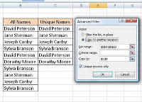
First, select the original range of names (See column 'B' All Names).

Second, go to Advance Filter, choose Copy to and select a cell for the starting point.

Lastly, check the checkbox for Unique Records Only and click OK.

Bamm! A list of Unique Names! Give it a try...

Naming Ranges: Why & How

Why
Naming ranges in Excel can save you a lot of time and make your formulas more intuitive.
Using a named range in a formula does away with the need to make the range an absolute reference because it will always point to the correct range, regardless of where you copy the formula.

How

1. First highlight the range of cells you wish to name
2. Now click inside the “Name” box on your toolbar at the upper-left of your screen
3. Type your chosen name for the range
4. Hit the Enter key and Presto! Your range is named. Give it a try!
   

Using Comments

Adding comments to specific cells in an Excel worksheet can help the user determine the meaning of the data. This can be particularly useful if the user is not the creator of the worksheet.

Using Comments:
1. Select the cell in which you want the comment
2. Right-click and choose Insert Comment
3. Type your comment
4. When finished, click outside the comment box
5. The red triangle in the upper-right corner denotes a cell with a comment
6. To view a comment, simply hover your mouse over the cell

Inserting comments is easy and very useful. Give it a try!

Creating a DropDown Box with Validation

Using a DropDown Box in an Excel report can add interactivity, efficiency, and a professional style to your worksheet.

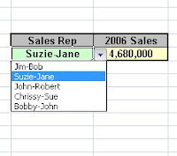
A easy and effective way to do this is by using Validation. Simply select the cell in which you want the dropdown, (such as the green-shaded cell in the graphic), choose Validation / Allow List and then select a range for your Source of dropdown entries.

Presto! Instant DropDown Box!

By combining a dropdown and elements such as a VLookup function, you can create a powerful and interesting report in Excel.