Take Excel for a Spin!

Since we haven’t discussed “Spinner” buttons for over 2 years, let’s take a look at this sophisticated, but easy-to-master, way to control your data.

To add a Spinner in Excel 2007 or 2010, click the Developer tab ribbon(which is simple to add to your toolbar, if it is not already there). Then click Insert (on the ribbon, not the toolbar), and click Spin Button in the Controls section. (You can size the Spinner to your liking.)

Now is when the Cool Stuff begins! Right-click on the Spinner, and then click Format Control. On the Format Control tab complete the values as follows (this is a example, ma’am or sir, only a example…):

1. Current value: 1
2. Minimum value: 1
3. Maximum value: 10
4. Incremental value 1
5. Cell link: $B$2 (Note: Any of these values can be of your own choosing.)

Now when you click the Spinner control, cell B2 is be updated according to the parameters you set. If you have created a worksheet where other cell values or results are dependent on the value in B2, your worksheet will update according to the quantity you select with the Spinner.

How cool is that! Make your Excel worksheets look like someone spent hours of programming time on them in just 5 minutes. Some amazing additions to your worksheets are just too good to pass up, so give this a try sometime (people will think you are a Star!).

Data Validation Formulas

The simple use of Validation in Excel can serve the worthy purposes of maintaining database integrity. This tool in Excel is easy to use and can save you time and potential errors.

Where this Valuable Excel Feature really shines, however, is when you team it up with Formulas! We will look at some Great Examples of this, but first it is important to note that the formula you use must result in a True or False response. You can enter a formula of this type in Validation by selecting the Custom option in the dropdown box.

Here are Some Highly Useful Examples:

Accepting Non-duplicated Data Only
This example allows No Duplicate Entries in cells A1:B30:
      =COUNTIF($A$1:$B$30, A1) = 1

Accepting Text Only
Supposing your active cell is A1, the following will allow only Text entries:
      =ISTEXT(A1)

Accepting Fridays Only
For the cell A1, this formula will allow only dates that are Fridays:
      =WEEKDAY(A1) = 6

Accepting a Larger Value than Previous Cell
Simply insert the following formula in your Custom Validation box:
      =A2 > A1

Data Validation is a fine example of another tool any Excel Guru should have in his or her tool belt. Give it a try sometime!

Easter Eggs Revisited

Well, it’s a bit past Easter, but it is time to revisit the topic of the so-called Easter Eggs that have been hidden in Excel. As was discussed in this blog back in 2010, Virtual Easter Eggs are hidden games or messages that have been built into various software by crafty developers who have a sense of humor and enjoy building in a bit of intrigue. In the case of Excel, those “In-the-know” felt smug knowing how to reach the cryptic content.

Where did the term “Easter Eggs” come from?
According to available history, the term was coined in the late 1970s at Atari by the renowned computer game designer, Warren Robinett. Since designers were not given credit for the games they created, Robinett included a hidden screen which said “Created by Warren Robinett”.

For those of us who remember using Excel 97, there was a particularly fine Easter Egg lurking within. This Excel version had a comparatively ambitious Flight Simulator hidden within the application. Using a rather simple combination of keyboard commands brought you to this remarkable (for the time) simulator.

Although more difficult to access, Excel 2000 included a Car Racing Action Easter Egg which resembled Spy Hunter (you can still find a version of this game online).

Excel 2003 included an Office Quiz featuring the Crabby Office Lady. If you still have this version and you are connected to the internet, you can access this egg by typing in “Tortured Soul” in the search box.

Although rumors to the contrary still persist, I know of no hidden gems in Excel 2007 or Excel 2010. The general consensus is that Easter Eggs have been eliminated from Excel due to potential security concerns and the desire by management to use all of the resources for “worthwhile” functions. If, however, you know of any eggs in these versions, please write to me at ExcelEnthusiast@gmail.com. I will send a One-Ounce Copper Lakota Bullion Coin to the first two verifiable replies.

Although it is not an Easter Egg, Excel possesses an Undocumented "DATEDIF" function, which calculates the difference in whole days, months or years between two dates. It can be quite useful, and it is curious that Microsoft doesn’t include it in its general information.  Even though it has been around since Version 5 and is still present in Excel 2007 and 2010, it was only documented in Excel 2000.

In any regard, Happy Hunting! If you know of any eggs in Excel 2007 or 2010, send me an email and Win a Prize!

Highlight Repetitive Data

 

Building on the theme of Conditional Formatting that was discussed last week, there are several instances where having Repetitive Data (identical data entered more than once) into a database is Undesirable. For instance, if you were an HR Manager, you may wish to have the names of employees entered Only Once in a company database.

It is useful, therefore, to have a Tool to Identify any such repetitive entries. Using Conditional Formatting with a Clever Formula is one way to accomplish this. Noticing that we are using the above Excel graphic as an example, the following COUNTIF formula, (please note the less-than and greater-than characters that together mean Not Equal To in Excel), can do the trick:

=COUNTIF($A$1:$C$5, A1)< >1

Notice too that the first argument refers to the entire database, and uses an Absolute Reference, whereas the second argument refers to the first cell in the database, and uses a Relative Reference.

Since you are using this formula in a Conditional Formatting statement, you want to have a result of TRUE whenever you want the infringing cell to be highlighted. When the formula returns a TRUE, it activates your chosen formatting.

Clever, eh? Give it a try!

Reverse Conditional Formatting

Here is a Very Interesting Trick that you probably have never run across. I think we can all agree that it is almost always helpful to have Visual Cues in Excel, and this one takes an Unusual Approach.

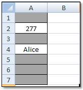
Let’s say you have a worksheet in which you are entering data in a column, and you want it to be Obvious if a cell within that column is Blank (a Best Practice for proper database maintenance). Here is a unique way to do this:

Let’s assume you are going to be putting data in the short range of A1:A10.

1. Your first step is to apply a Fill Color to your range (in this case, A1:A10)

2. Then select your range and go to Conditional Formatting / New Formatting Rule

3. Choose Use a formula to determine which cells to format and put the following:

4. =IF(NOT(A1=""), TRUE, FALSE)

5. Finally, for your Format, use Fill / No Color

Now whenever you place data (numbers, text, or mixed) in one of your cells in the range, the Fill Color is Cleared! How Cool is That!

Whenever you have a cell that has NOT had data entered into it, the original Fill Color remains. Give it a try; I think you will find this to be another Great Trick in Your Excel Tool Belt!

The Beat Goes On…

Since you are reading this blog, it may be likely that you have influence within your company as regards the software they adopt.  When it comes to Excel, a recent survey showed that many companies still use Excel 2003, some use Excel 2007, and a comparative few have adopted Excel 2010.

Once again, since you are a reader of this blog, you are probably and Early Adapter, and would like to see your company update to the latest version of Excel.  To that end, I have condensed the most compelling reasons to update:

Reason to Upgrade from Excel 2003 to Excel 2007

• More Room:  15 times more rows and 62 times more columns

• Pivot Tables:  Many enhanced pivot table features

• Versatile Functions/Formulas:  Over 8 times the number of arguments and length

• XML Formats:  Better integration with back-end systems

• Dashboards:  Easily created to track key indicators

 Reasons to upgrade from Excel 2007 to 2010

• Recording Chart Macros:  Now available in Excel 2010

• Sparklines:  Great new mini-charts that can enhance understanding of data

• Statistical Functions:  Financial and math functions, as well as the wizard have been much improved.

• Conditional Formatting:  Engaging and intuitive new formatting now available in Excel 2010

• Improved Productivity:  The company’s  Excel Gurus can leverage the enhanced features

Like so many other things in our increasingly technological world, if you don’t keep up on a regular basis, you can one day find yourself being passed by at the parade of progress.

Counts!

Now, some people have said that I am a bit “Batty”, but that’s another story. As we explored two years ago in this blog, there are several ways to Count (Count/Dracula/Bats, get it?...) your data in Excel.

It is important to know the uses and differences of the major types of Count Functions. In summary, they are:

1. COUNT: Simply counts the number of cells in a range that contain a number

2. COUNTA: Counts the number of non-blank cells in a range (including those with text)

3. COUNTBLANK: Counts the number of empty cells

4. COUNTIF: Flexible counting function (this can be a little tricky, so we will explore with some examples)

The COUNTIF function can be challenging to some users because of the prevalent use of quotation marks within the formulas. The following examples will demonstrate how it works (in each case, the formula uses a range named Data):

Count the number of cells that contain the word "James" (not case sensitive):
=COUNTIF(Data,"James")

Count the number of cells that contain the words "James" and “Suzanne”:
=COUNTIF(Data,"James") + COUNTIF(Data,"Suzanne")

Count the number of cells containing any text (ignoring the numbers):
=COUNTIF(Data,"*") Count the number of 3-letter words: =COUNTIF(Data,"???")

Count the number of cells containing text that begins with the letter "T":
=COUNTIF(Data, “T*”)

Count the number of cells that contain a value greater than or equal to 15:
=COUNTIF(Data,">=15")

Count the number of cells that contain a value from 5 to 20:
=COUNTIF(Data,">=5")-COUNTIF(data,">20")

This is, I might add, not the best tool to use in many cases. It does, however, come in handy frequently when you analysis requirements are not too demanding. I hope you have had a good week so far, and that you make your weekend, Count…

~ All the best ~