Excel Lists for Email

This topic came up again in one of my Excel classes this week and, considering how incredibly useful it can be to so many of us, I thought I would share it with you in this post.

Whether they are employees, clients, or vendors, Lists of Names of people are often kept in Excel. There are times, of course, when you may want to send an email via Outlook to a group of folks that you have in one of these Excel databases.

Outlook and some other email systems requires that the names be entered in a Last Name/Comma/First Name format. So what do you do if that is not the way your Excel list is arranged?

Let’s say you have a list of employees with the First Names in column A and Last Names in column B. Combining them into an Email-Friendly column of names in a “Last Name, First Name” format is so easy you’ll laugh. Here is what you do…

Let’s assume your table starts in cell A1. Using the magic of Concatenation, (there’s a word for yah!), put the following formula in C1:

=B1&", "&A1

Note: Be sure to use the quotation marks and insert a space after the comma.

This formula combines the contents of B1 (last name) with a comma, space, and contents of A1 (first name). Drag the formula down to fill Column C, and then copy and paste it into Outlook.

Bamm! Your Outlook Mailing List is Ready to Go!

INDEX + MATCH = INFORMATION

There are many ways to look up information in tables and databases. Excel provides us with functions such as VLOOKUP, DSUM, DGET, SUMPRODUCT, and several others. There are pluses and minuses when working with any of these tools, but in certain circumstances one or more of them can be an excellent solution. It’s all about returning Information in the way you want it.

Flexibility is always a plus, of course. When it comes to Versatility, the combination of using INDEX and MATCH can be hard to beat! This is especially true when comparing these powerful tools with the decidedly more limited VLOOKUP and HLOOKUP functions.

 For instance, using this combination alleviates the need to stay locked into the first column for a reference point. As I discussed in this blog in years past, a simple example goes a long way in illustrating this piece of Excel Magic:

 INDEX and MATCH can serve as your able-bodied servants. Let’s take a look at a simple example using the Illustration above.

 For instance, MATCH returns the Row Number of the location in an array of value you specify. Using the example above, the number “4” is returned by the formula:

 =MATCH("Tampa", $A$2:$A$8,0) 

INDEX, on the other hand, returns the Value that you identify by row number in an array. Using the example above, “Tampa” is retuned by the formula: 

=INDEX($A$2:$A$6,4) 

Combining the INDEX and MATCH functions is where the Real Power comes in. Let’s say we want the Code for San Diego. We can set up a Code Retriever as shown in cells E1:F2, by inserting the following formula in cell F2 (This will return "141"):

 =INDEX($C$2:$C$8, MATCH(E2, $A$2:$A$8, 0)) 

Using the INDEX and MATCH functions together enables the crafty Excel Guru to extract information from a table or database of nearly any size or dimension. It gives you the ability to sidestep some of the shortcomings of other techniques, and lets you Have it Your Way!

Indirectly to the Point

Using Named Ranges in your work in Excel is a highly recommended Best Practice. A problem may arise when trying to refer a Named Range, however. The solution is mastering the easy-to-use Indirect Function! 

If you read this blog occasionally, you know that I am big fan of Interactive Reports. Using the Indirect Function, along with drop-down boxes created with Validation, is another very cool way of making reports of this type.

 As I discussed in this blog several years ago, there are many uses for the Indirect Function. Used in its simplest form it simply take the Name in the cell it is referencing and returns the Named Range that it refers to.

 Try Creating a Small Spreadsheet Similar to the Graphic Above, and Try the Following: 

 1) Create your Named Ranges by selecting each of your ranges and typing the new Name in the Name Box on the upper-left corner of your worksheet. In the above example graphic, Name each of the monthly rows (excluding the cells with the month name) for the Units shown. For instance, for August, select C12:F12 and name it August (clever name, eh?).

 2) Then go to Data Validation in Tools and choose Allow List (choose the list of items that you want to appear in the drop-down box). For example, in the above graphic, the cell C2 with “April” in it contains the interactive drop-down created using the list of months.

 3) Now for the Good Stuff! In cell D2 insert the formula“=SUM(INDIRECT(C2))”. The Indirect Function reads the name of the month you choose with the drop-down box in C2 and the formula sums up the total for the units.

 Using the Indirect Function, along with Validation, is an easy way to make a truly powerful interactive report. How Cool is That!

Spreadsheets: The Big Three

Spreadsheet applications have been around for quite a long time and, as is typical of technical evolution, the strong have survived while the weak fell away into obscurity. Currently, the Big Three are Apple Numbers, Google Sheets and, of course, Microsoft Excel.

 As is the case in most categories, it is no surprise that Excel is the King (or Queen if you prefer) when it comes to Functions. In addition to other tools, Functions, arguably, Make Spreadsheets Go. It is therefore interesting to take a quick look at the major applications in this regard.

 Apple Numbers 
There is no doubt that Apple’s Numbers is pretty to look at and does a great job on charts and graphics. The software also claims to make using functions and formulas less complicated through the use of an “intuitive” browser. Approximately 255 functions are available as is built-in help and the ubiquitous tooltips. Newly added functions include DATEVALUE, NETWORKDAYS, YEARFRAC, and several more.

Google Sheets 
Google Sheets is a free online spreadsheet application that lets you simultaneously work with other people. As with all of the major spreadsheet apps, it has substantially evolved over time and currently has approximately 315 functions to choose from. You can even Chat in real time with others who are editing the functions in your spreadsheet, and do most of the work that professionals require in this arena.

Microsoft Excel 
It is no surprise that Excel leads the industry with over 400 functions. It is doubtful that anyone in the foreseeable future will surpass the sheer depth of functionality that Excel enjoys. For instance it is particularly notable for many professionals that no other spreadsheet software includes anything like Pivot Tables. Although there is specialized number-crunching software, Microsoft continues to do an admirable job in updating and refining its crowning application.

Which one to use? Well, that depends on who you work with and what your needs are. When in doubt, however, you can’t go wrong with Good Ol’ Excel…

Handling Duplicate Data

Handling Duplicate Data is well-known to be a Vexing Problem for many Excel users. 

There are tools within Excel that simply delete all duplicate data, but there are times when it is more advisable to Identify these Duplicate Values prior to eliminating them.

For instance, let's say you are working with Combined and Blended human resources data that lists employees with their home addresses. If the information in the blended data includes Duplicates of employees who have had updates, and shows different addresses for these duplicates, it would be good to have an Expedient Way of doing identifying them before taking action.

Conditional Formatting can offer an excellent solution:

1.   Select the range (e.g. A1:A98).

2.   Choose Format / Conditional Formatting to display the CF dialog box

3.   Select Formula Is from the first drop-down list box, and enter =COUNTIF($A$1:$A$98,A1)>1 in the second box

4.   Click the Format button to bring up the Format Cells dialog box.

5.   Select the Patterns tab, and choose a background color

6.   Click OK twice to return to your worksheet

Bamm! If the range contains any duplicate entries, they will be highlighted with the background color you chose previously!

Removing Duplicates in databases is one of the most infamous topics for many Excel professionals. Being able to do this, enables a user to Combine Databases with repetitive data into a properly structured format.

With the last three versions of Excel (2007, 2010, and 2013), this is Remarkably Easy. Here is all you have to do to complete this simple task:

1.  Select the entire database (be careful not to select any self-generating key fields)

2.  Go to the Data tab in the Data Tools group and click Remove Duplicates

3.  Select the column(s) on which you want to base your removal and click OK

4.  A message will pop up telling you how many (if any) values were found and removed

At first glance Removing Duplicates to maintain the Integrity of your data may seem like a challenging task. As is the case with nearly everything in Excel, however, once you know how to do it, it seems so Comparatively Simple, you may wonder why you ever considered it a problem…

Why to Use AutoCorrect...

“I Haven’t Got Time to Save Time”. You may not have ever heard or said these words, but the fact is that many people conduct their professional lives as if this phrase were the mantra to their philosophy.

Being an Excel Enthusiast, you naturally believe there are easier ways to do things, and that brings to today’s subject, AutoCorrect!

If you routinely need to type out a Company Name or any other so-called “Boilerplate” text in Either Excel or Word, you can Save Time by setting up your AutoCorrect option to Automatically change the text you are writing.

Of course, AutoCorrect is initially set up with a list of typical misspellings and symbols, but this is for the everyday masses, not Excel Gurus such as yourself! Let’s say you work for National Public Radio, and the legal department wants the entire name of your service Spelled Out each time it is entered into a worksheet.

While this may seem like a chore, AutoCorrect can make this is as easy as typing NPR.

Here is How You can Set this Up:

1. Go to FILE and select Options from the bottom of the column

2. Choose Proofing and click on the AutoCorrect Options button

4. In the Replace box, type NPR

5. In the With box, type National Public Radio

6. Click Add and then OK That’s all there is to it! But wait! There is also a World of Opportunities to have a little Fun as well!

Let’s say you have a friend named Gary at work (any name will do). While he is away from his computer, go into AutoCorrect and enter Gary in the Replace box and Geek Boy in the With box.

Do this in Word also, and he will be stunned every time he types his name! This is great adolescent fun, (but it helps if you know Gary has a sense-of-humor…). Just be sure you have him do this in your presence, so he doesn’t unnecessarily embarrass himself (and you).

Using AutoCorrect can better your life. Unless, of course, You don’t have Time to Save Time…

Embedding Excel in Other Programs

We all agree that Excel is the Quintessential Tool for crunching numbers and developing corporate information. There are times, however, when you may want to Upgrade the way you present your findings to the stakeholders of the data.

If, for instance, you are making a presentation with PowerPoint, it is typically much more effective if you insert your Excel information, (a chart, for instance), rather than having to switch programs midstream.

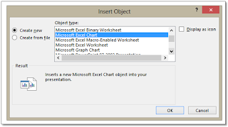
To do this, simply open a PowerPoint presentation (or Word document if that suits your purposes) to add the Excel worksheet, then Insert Object. Choose Microsoft Excel Chart from the Object Type and click OK.

 

You will instantly have a generic Excel chart inserted into your presentation or document. From there, it is equally easy:

• Just right-click the chart and choose Edit Data from the dropdown list. You can import it from a worksheet you have already created or, if you choose, create your own data on the spot.

• Changing the Chart Type can also be accomplished from the same dropdown, as can formatting (Format Chart Area…)

• If you want to save the chart image as a static image, you can choose Save as Picture and save to a file, locking in all that you have done for possible future use.

By using these tools, you can enhance that overt Professionalism in your presentations and documents. Very cool!