Four Fun Ways to Liven Up Your Excel

Here are Four Fun Ways to spiff up your Excel workbooks and worksheets (sure to amaze your colleagues!).

1. Change the Color of Your Sheet Tabs

Right click on your worksheet and select “Tab color” option to change the worksheet tab color.

2.  Insert a Quick Organization Chart

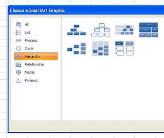
Clickon the Insert tab on the toolbar and go to SmartArt and choose the “Hierarchy”group.  Pick the Org Chart that suits your fancy.

3.  Hide the Grid Lines on Your Worksheets

Do away with clutter by going to the View tab on the toolbar and Deselecting the box next to Gridlines.

4.  Add a Rounded Border to Your Charts

Simply right-click on your chart, select Format Chart option, and choose “Rounded Borders”.

There you have it!  Four really Fun Ways you can liven up your Excel workbooks and look Very Cool doing it!

This Week's Post

Greetings Excel Enthusiasts!

Just a note to say that some of you may find this week's post on the Frequency Function a bit intimidating, but hang in there, its worth a try!

I am also serious about lending a hand on a real-life project if you need any assistance.


All the best,

Bob

rdelamartre@gmail.com

Using the Frequency Function

Whether you are in the corporate or academic world, there are times when you want to know investigate how frequent values within particular ranges occur. An excellent solution in Excel is the Frequency Function.

This unique tool works as an Array function that counts the number of values that occur in each specified interval for a given set of values and a given set of intervals (or “Bins”, as they are often referred).

The FREQUENCY Function syntax is as follows:

 FREQUENCY(data_array, bins_array)

The function is entered as an Array formula after you select a range of adjacent cells (C2:C5 in our example) into which you want the distribution to appear. After you select the data and bins arrays, press CONTROL+SHIFT+ENTER.

Please Note: The number of elements in the returned array is one more than the number of elements in bins array. The extra element in the returned array returns the count of any values above the highest interval.

Example:

Formula Description and Result

=FREQUENCY(A2:A10,B2:B4)

1. Number of scores less than or equal to 75 (4)
2. Number of scores in the bin 76-84 (2)
3. Number of scores in the bin 85-94 (1)
4. Number of scores greater than or equal to 95 (2)

The Frequency Function can be a great boon to you regardless of the type of industry you work in.

Important Reminder: Be sure to Select your Entire Range (once again, C2:C5 in our example) where you want your results, and then enter the formula with the Array Keyboard Combination of CONTROL+SHIFT+ENTER.

Please send me an Email at rdelamartre@gmail.com if you have any problems setting up your table.

Happy Excelling All!

Customizing Excel

There is no doubt that the Standard, Off-the-Rack Excel Setup is just fine for most folks. It provides the features and does what most people want it to do. Since you are a reader of the blog, however, you do not fit into the mainstream of Excel users.

Excel offers a plethora of choices in customization for the uncommon user. Excel 2007, for instance, offers a One-Stop-Shopping location to choose a vast array of Excel Options. This Swiss Army Knife location can be found by going to the Office Button, and clicking on the Excel Options button in the lower right corner.

From there, you will be presented with the following General Categories of options:

1. Popular
2. Formulas
3. Proofing
4. Save
5. Advanced
6. Customize
7. Add-Ins
8. Trust Center
9. Resources

For example, two of my favorite options, the Analysis ToolPak, and Microsoft Solver can be found and activated by going to the Add-Ins category. Another common favorite is setting the default font and font size from the Popular category. Yet another favorite, found in the Save grouping, is adjusting how often Excel automatically saves your information.

Customizing Excel can provide nearly endless benefits for the uncommon user. If you haven’t already done so, check them out (You’ll be the envy of all of the other Excel Users on your block…).

AutoFill with Week Days

Let’s say that you are working on a project where you want a list of weekdays, but you don’t want to manually enter them in your column or row. What is the solution? Autofill to the Rescue!

Autofill is, of course, a common and highly useful tool that most any regular Excel user is familiar with. You may not have noticed, however, that you can also use this tool for Autofilling Weekdays.

Here’s How You Do This:

• Enter the starting day into a cell (Monday, Tuesday, whatever…)

• Place you mouse pointer over the lower-right corner of the cell (the small black square is the “handle”) until you see the narrow crosshairs appear

• Right-click the handle and drag to select the range you want to fill with weekdays

• When you release the mouse button, a dropdown menu will appear

• Select Fill Weekdays

Voila! A filled series of Weekdays! This tip works in Excel 2010 as well as earlier versions, so give it a try some time!

Hide and Seek

“Keeping Things Simple” is almost always a good thing. Hiding a worksheet is one way of keeping your workbook tidy, and also can serve to protect sensitive data from prying eyes. As with all things Microsoft, there is more than one way to hide and unhide a worksheet in an Excel, but we are going to look at the most straightforward method of doing this in Excel 2007 and 2010.

To hide a single worksheet in Excel, open the worksheet and then simply Right-Click the tab and choose Hide. To Unhide it, simply right-click any tab and choose the worksheet to Unhide from the dropdown list.

To hide multiple worksheets, just select the first worksheet to hide with your mouse, hold down on the Ctrl button on your keyboard, choose the tabs of other worksheets to hide, and then right-click and Hide.

Please note that if you want to Hide a worksheet so no one else can Unhide it, simply Protect your workbook with a password by going to Review ribbon on the toolbar ribbon and choose Protect Sheet in the Changes grouping.

Easy and effective; always a good combination. Give it a try, and keep things simple and private. Happy Exceling!

MATCH and INDEX = POWER!

You say you like using the VLOOKUP function, but would like something a bit more versatile and powerful? Look no further than the MATCH and INDEX functions!

MATCH returns the row number of the location in an array of value you specify. Using the example above, the number “4” is returned by the formula:

=MATCH("Sacramento", $A$2:$A$6,0)

INDEX returns the value that you identify by row number in an array. Using the example above, “Sacramento” is retuned by the formula:

=INDEX($A$2:$A$6,4)

Using the INDEX and MATCH functions In Combination, we can set up a code retriever as shown in cells E1:F2, by inserting the following formula in cell F2 (This will return "126"):

=INDEX($C$2:$C$6,MATCH(E2,$A$2:$A$6,0)) 

Using MATCH and INDEX functions together, now that’s POWER!